グラフィカル連鎖モデルに基づく因果推定法の遺伝子発現プロファイルへの適用

全文

(1)2005−BIO−3（8） 2005／12／22. 社団法人情報処理学会研究報告 IPSJ SIG Technical Report. グラフィカル連鎖モデルに基づく因果推定法の遺伝子発現プロファイルへの適用油谷幸代 1, 斉藤秀 1,2, 堀本勝久 1 1 2. 東京大学医科学研究所バイオスタティスティクス人材養成ユニットインフォコム（株）バイオサイエンス部. 概要グラフィカル連鎖モデルに基づいて、遺伝子発現プロファイルから異なった細胞状態で発現する遺伝子群の因果関係を推定する方法を開発した。細胞周期 G1, S, G2, M 期で特徴的に発現する 619 遺伝子の発現プロファイルデータに適用したところ、四つの異なった細胞状態で 50 群に分類された遺伝子群間の因果関係が推定され、特に、隣接する状態としない状態の細胞との間で因果性を示す遺伝子群が異なることが推定された。. A graphical chain modeling approach for analyzing gene expression profiles Sachiyo Aburatani1, Shigeru Saito1,2, Katsuhisa Horimoto1 1 2. Laboratory of Biostatistics, Institute of Medical Science, University of Tokyo Bioscience Department, INFOCOM CORPORATION.. ABSTRACT A procedure of the chain graph modeling is designed for analyzing the expression profiles of genes that can be classified into several blocks in a natural order. The newly designed procedure for graphical chain modeling was applied to 619 expression profiles of cell-cycle related genes in yeast, which were experimentally identified to be transcribed in order of four cell-cycle phases, G1, S, G2, and M. By the application, 619 genes were classified into 50 clusters, and a chain graph of 50 clusters in the four blocks was constructed. One of the remarkable features is a distinctive relationship of clusters between neighboring and non-neighboring phases. The merits and pitfalls of the graphical chain model are discussed in terms of the application to the field of molecular biology.. INTRODUCTION Cell integrity and survival strongly depend on the precise coordination of the unidirectional transitions between cell cycle stages. Cell cycle–dependent mRNA variations have been observed for genes involved in various cellular processes, including control of mRNA transcription [28], responsiveness to external stimuli [29], and subcellular localization of proteins [19]. In addition, the activity of cell cycle–regulatory proteins is required for normal DNA repair [18, 25], meiosis [15], and multicellular development [12, 22]. These observations associated with the cell cycle make it an attractive model for studying the genome-wide regulation of gene activity. Indeed, microarray technology can now provide comprehensive results for a genome, and thus reveal the novel functional and physical organization involved in coordinating cell-cycle gene regulation [5, 21]. About 800 genes related to cell cycle regulation were identified by using periodicity and correlation algorithms [21]. In order to infer a regulatory relationship on a genomic scale, we have recently developed an approach to infer a regulatory network from gene expression profiles on a genomic scale, in combination with graphical Gaussian modeling (GGM) and hierarchical clustering [14, 23]. Among the graphical models, GGM is the simplest structure in a mathematical sense; only the inverse of the 1 −51−.

(2) correlation coefficient between the variables is needed. GGM infers only the undirected graph, instead of the directed graph showing the causality in the Boolean and Bayesian models, and therefore, GGM can be easily applied to a wide variety of data. Since straightforward applications of statistical theory to practical data fail in some cases, GGM frequently fails when applied to gene expression profiles. This is because the profiles frequently share similar expression patterns, which indicate that the correlation coefficient matrix between the genes is not regular. Thus, we have devised a procedure, named ASIAN (Automatic System for Inferring A Network), to apply GGM to gene expression profiles, by a combination of hierarchical clustering [2, 3, 24]. First, the large numbers of profiles are classified into groups, according to the usual analysis of profiles. To avoid the generation of a non-regular correlation coefficient matrix from the expression profiles, we adopt a stopping rule for hierarchical clustering. Then, the relationships between the clusters are inferred by GGM. Thus, our method provides a framework of gene regulatory relationships by inferring the relationships between the clusters [1, 23], and provides clues toward estimating the global relationships between genes on a genomic scale. In this paper, we describe a procedure for analyzing expression profiles that can be naturally grouped and ordered from prior biological knowledge, by graphical chain modeling [6, 26, 27], based on the ASIAN procedure. We apply our procedure to the cell-cycle related genes that can be divided into four blocks, and describe how graphical chain modeling can be used to provide an easily interpretable empirical analysis of the factors influencing the regulatory relationships of the cell-cycle. In particular, the linking of the four blocks into a chain graph is expected to provide new insights into the direct and indirect associations between gene groups in distinct blocks.. MATERIALS AND METHODS Graphical Gaussian Model The concept of conditional independence is fundamental to graphical modeling. The conditional independence structure of the data is characterized by a conditional independence graph. In this graph, each variable is represented by a vertex, and two vertices are connected by an edge if there is a direct association between them. In other words, two vertices are not connected if they are conditionally independent, given all the other variables. The construction of multivariate models based on the concept of conditional independence for continuous variables was initiated by Dempster [8], under the name “covariance selection models”. However, the paper did not mention the idea of using a graph to summarize the results of an analysis. The report by Darroch, Lauritzen and Speed [7] combined the ideas of conditional independence and log-linear models, and used the intimate connection between them to define graphical models. Thus, the graphical Gaussian models can be easily interpreted using the Markov properties of the associated independence graphs. Furthermore, the iterative algorithm for computing maximum likelihood estimates, described by Speed and Kiiveri [20], enables us to analyze practical data. For more details about the rapid developments in this area, see [9, 17, 27]. Graphical Chain Model Graphical chain model is one of the probability models for multivariate random observations whose independence structure is captured by a graph. A graph Γ = (V, E) consists of a set of vertices V, representing the variables, and a set of edges E, representing the association between pairs of variables. E is a set of ordered pairs (A, B), A, B ∈ V. A chain graph is based on a partition of V into disjoint subsets: V = V1 ∪ V2 ∪ …∪ VT. The subsets are called blocks or chain components. Edges within blocks are undirected reflecting systematic associations and edges between blocks are arrows pointing from blocks with lower index numbers to those with higher indices. A graphical chain model displays the independencies between variables conditioned on all the other variables in the current and previous blocks. In a graphical chain model, any direct association between two variables in the same block is assumed to be non-causal and is represented by an undirected edge (line) in a graph. Any direct association between two variables from different blocks is assumed to. 2 −52−.

(3) be potentially causal and is represented by a directed edge (arrow). The absence of a line or arrow between two variables in the graph indicates that there is no direct association between the variables, i.e. the variables are independent after controlling for all the other variables in the same and previous blocks. The first step when fitting a graphical chain model is to partition the variables into a number of ordered blocks. The variables in the first block are viewed as purely explanatory variables, whereas the variables in the second and subsequent blocks are viewed as responses to the variables in the preceding blocks and as explanatory variables for the variables in the succeeding blocks. The graphical chain model is fitted in a number of stages. First, the significant direct associations between the variables in Block 1 are determined. For each pair of variables the null hypothesis when tested shows that the variables are independent given all the other variables in Block 1 and the deviance statistics in graphical Gaussian modeling is used [9,11,27]. Second, the significant direct associations between the variables in Block 2 and between Blocks 1 and 2 are determined. Foe each pair of variables the null hypothesis when tested shows that the variables are independent given all the other variables in Blocks 1 and 2 and again the deviance statistics is used. The fitting continues, block by block, by determining all the significant direct associations between the variables in the current block and between all the variables in the current and previous blocks. The null hypothesis is now independence given the other variables in the current and previous blocks and again the deviance statistics is used. All these tests were carried out at the 5% level using the deviance statistics [9,11,27]. Application of Graphical Chain Model to Gene Expression Profiles The block in graphical chain model simply corresponds with the phase that is defined by biological knowledge, cell cycle phase in the present study. By the intact correspondence to graphical chain modeling, the variable is the gene that has expression profile of numerical values. However, since the expression profiles often show similar patterns, the genes are highly related with one another. Thus, hierarchical clustering is performed for the genes within each block as a preprocessing for the graphical chain modeling, and then, each gene cluster corresponds with the variable in the present procedure. The clustering, the estimation of cluster number, and the graphical Gaussian modeling are calculated by our ASIAN web site (http://eureka.ims.u-tokyo.ac.jp/asian) [2]. The details of the procedure are as follows. The genes within each block are grouped into some clusters. Since the metrics and the techniques in the clustering depend on the data and interests [13], the hierarchical clustering is performed with 15 pairs of three metrics (correlation coefficient between profiles, Euclidian distance between profiles and Euclidian distance between Pearson's correlation coefficients of profiles) and five techniques (Single Linkage, Complete Linkage, UPGMA, WPGMA, and Ward's Method). The cluster numbers are estimated in the dendrograms in four blocks, which are constructed in (a), respectively. In estimation, the variance inflation factor is adopted as a stopping rule for expression profiles [14]: the threshold value is set to 10.0. In this step, we obtain clusters in each block, and the clusters are regarded as the variables in the blocks for further analyses. The average expression profiles are calculated according to the cluster estimation in (b). The average correlation coefficient matrix is calculated from them. The graphical chain modeling is performed for the correlation coefficient matrix of the valuables that correspond with each cluster. In the chain modeling, the association of the variables (clusters) within and between blocks is inferred by the graphical Gaussian modeling. Note that the average correlation coefficient matrix in (c) is not always regular. This indicates that the inference of association in (d) is impossible. Thus, we perform a heuristic analysis for selecting appropriate pairs of metric and technique in the application of graphical chain modeling. First, we perform the graphical Gaussian modeling for the average correlation coefficient matrices in each block, which are obtained by various pairs of metric and technique in (a) and (b), and then select the metric and technique pair by testing whether the graphical Gaussian modeling can be performed in each block. In the present analysis, 15 pairs of metric and technique are tested to select the suitable pair for the graphical chain modeling.. Expression Profile Data 3 −53−.

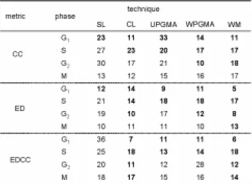
(4) We use the expression profiles of 796 genes measured at 77 conditions [21], which are identified to be related with cell cycle regulation. In the present analysis, we regard the cell-cycle as one sequential event of G1 phase to M phase. Thus, we select the genes specific to each phase, by excluding the genes that express in the intermediate stages. For this purpose, we classify 796 genes into clusters, and then extract the genes included in the clusters that are characterized to four phases with 1% significance level [1]. As a result, 619 genes are selected and are divided into 242 in G1 phase, 128 in S phase, 177 in G2 phase, and 72 in M phase.. RESULTS Clustering of Genes in Four Phases Table 1 shows the test for 15 pairs of metrics and techniques in hierarchical clustering in the preceding subsection (a) and (b). In three pairs among 15 pairs, the graphical Gaussian modeling can be successfully performed for the average correlation coefficient matrix in four phases; the pairs are Euclidean distance between profiles and Ward’s method, Euclidean distance between correlation coefficients and complete linkage, and Euclidean distance between correlation coefficients and Ward’s method. In other pairs, the graphical Gaussian modeling fails because the independency between gene clusters is not observed within each phase but between four phases. Thus, the pair of Euclidean distance between correlation coefficients and Ward’s method seems to be suitable for the hierarchical clustering for the large number of genes with many similar patterns in the graphical chain modeling. Table 1 Selection of metric and technique pairs in hierarchical clustering for graphical chain modeling. Although the genes in four phases are subjected to estimate the cluster number with the common threshold (VIF=10.0) for the stopping rule, the cluster numbers differed among the four phases by the hierarchical clustering with the Euclidean distance between correlation coefficients and Ward’s method. The largest and smallest numbers of clusters are the genes in S phase and those in G1 phase, respectively.. Independence Graphs for Each Step of the Analysis An interaction graph for each step of analysis for four cell-cycle phases is shown in Fig. 1. To extract characteristics from the graph, the following two simple rules are often helpful: (a) any non-adjacent pairs of variables that are not joined by a single edge are conditionally independent given the remaining variables in the current and previous blocks; (b) a variable is independent of all the remaining variables in the current and previous blocks after conditioning only on the variables that are adjacent (joined by a single edge) to it. Furthermore, since the gene expression profile can describe only relationship between the transcriptional factors and their regulating genes in a strict sense, the clusters including the transcriptional factors are selected within each block.. 4 −54−.

(5) In all graphs, there are many edges between clusters, irregardless of edges within and between the phases. In Fig.1, therefore, we focus on the clusters without the association. The association within the phases is strong (Figs 1(a), (b), (d)) except for M phase (Fig. 1(f)). The numbers of clusters with no edge are 1 of 6 cluster pairs in (a), 7 of 36 pairs in (b), 2 of 10 pairs in (d), and 4 of 6 pairs in (f). Since the number of genes in clusters including the transcription factor in M phase is relatively small to the cluster number, the genes with the direct association of transcriptional factors may be scattered in the other clusters. In comparison with the association within the phases, the fraction of cluster pairs with no edge between phases slightly increases; 11 of 36 pairs in (c), 23 of 65 in (e), and 21 of 72 in (g). In addition, the fractions show almost similar degrees in the respective phases. Indeed, the fractions in (e) are 6 of 20 pairs between G1 and G2 phases and 17 of 45 between S and G2, and those in (g) are 5 of 16 between G1 and M, 10 of 36 between S and M, 6 of 20 between G2 and M. In summary, the conditional independency of cluster pairs within phases is weaker than those between the phases, but the cluster pairs between the phases share similar degree of conditional independency.. Fig.1 Steps of graphical chain modeling in the four cell-cycle phases. The associations between clusters including transcription factors are drawn. The cluster is denoted by Cij: i (= 1, 2, 3, 4) corresponds to G1 phase, S phase, G2 phase, and M phase in the natural order of the cell cycle, and j corresponds to the number of clusters including the transcription factors shown in Table 2, in each phase. The associations within blocks are indicated by solid lines, and those between blocks are denoted by arrows.. Construction of Graphical Chain Model The chain graph presented in Fig. 2 shows the direct and indirect associations of each cluster in the four phases. The chain graph in Fig. 2 is constructed first by combining the graphs in Fig. 1. However, since there are many edges and drawing them all on one chain graph would produce a mess or `spaghetti' pattern which would be difficult to read, the variables in Fig. 2 have been rearranged. The cluster pairs in different blocks with partial correlation coefficient of more than 0.3 are selected. The arrows are drawn between the thus selected clusters only in different phases. For example, since four clusters (C1,1, C1,2, C1,3, and C1,6) in G1 phase and 9 clusters (C2,6, C2,7, C2,11, C2,12, C2,13, C2,14, C2,15, C2,17, and C2,18) in S phase contain the transcription factors, the arrows are drawn from the clusters in G1 phase to those in S phase when the partial correlation coefficient is more than 0.3 in the graphical chain modeling. The direct association shows a similar degree between neighboring phases and between non-neighboring phases. For example, the numbers of direct associations of clusters are 3 and 4 between 5 −55−.

(6) G1 and S phases and between S and G2 phases, while those are 3 and 6 between G1 and G2 phases and between S and M phases. A remarkable association is found in M phase; the association between M and the other phases seems stronger than that between other pairs of phases. Indeed, the numbers of cluster associations are 6 and 7 between G1 and M phases and between G2 and M phases. This may be related with the fact that G1, S, and G2 phases are regarded as the interphase for the cell division in M phase. In other words, the gene groups in the three phases of G1, S, and G2 may be coordinately regulated to final event of cell division in M phase. Apart from the number of association, a striking feature emerges by focusing the cluster association in neighboring and non-neighboring phases. Between G1 and S phases, the associations are found between the clusters C1,3 and C1,6 and the clusters C2,7, C2,14, and C2,15, while the associations between G1 and G2 phases are found between the clusters C1,1 and C1,2 and the clusters C3,7 and C3,8. Thus, the clusters in G1 phase are separate in terms of the association between neighboring phase (C1,3 and C1,6) and between non-neighboring phase (C1,1 and C1,2). The separation of clusters is also found in the clusters of S phase, with only one exception (C2,14); the association between neighboring phase (G2 phase) is found in the clusters C2,6, C2,13, C2,15, and C2,18, and that between non neighboring phase (M phase) is in C2,7, C2,11 C2,12, and C2,17. Although the total associations between the neighboring and non-neighboring phases are similar, the cluster pattern with the association is distinct between them.. Fig.2 Graphical chain model of regulatory relationships in the cell-cycle. The associations between clusters including transcription factors and showing a partial correlation coefficient of more than 0.3 are drawn by arrows, according to the cell cycle order, G1, S, G2, and M, from the top to the bottom. The associations between neighboring blocks and those between non-neighboring blocks are indicated by solid and broken arrows, respectively.. DISCUSSION There are two major advantages of using the graphical chain model in analyzing gene expression profile data. First, all the results can be displayed in a simple mathematical graph. From this graph the structure of the associations for the whole system under study can be ascertained very easily. Thus, a chain graph is a very powerful tool for displaying the results of the analysis, since it is more straightforward to read than results presented in some tables. Second, using graphical chain models, the variables are partitioned into several blocks. This enables us to carry out analyses for each block and to assess the associations between all the variables in the study. The linking of these blocks into a chain graph then gives direct and indirect pathways between any variable and its potential determinants. In this paper we examined the direct associations between gene clusters in four cell-cycle phases.. 6 −56−.

(7) The present study reveals the different patterns of conditional independency in the clusters between four cell cycle phases. In particular, the total association between the four phases maintains at similar degree, but the separate cluster association is found between the neighboring and non-neighboring phases. These results will require considerably more analysis for a definitive resolution, but the graphical chain modeling approach provides new perspectives on the cell cycle regulation. Furthermore, these observations can not be reduced by only standard analyses of gene expression profiles such as the clustering, indicating that the graphical chain modeling is a useful tool for analyzing the expression profile data. It is well known that many phenomena are observed, which the biological events occur sequentially by coordinated regulation of some gene groups, such as the differentiation and the development. In addition, the gene expression profiles are frequently monitored as the time series data. According to the biological knowledge and the time intervals, the expression profiles can be grouped into some blocks. Although the definition of blocks in some cases depends on the biological knowledge with some ambiguity and there are many intermediate stages between distinctive biological phenomena, the inductive modification of the graphical chain modeling approach from the analyzed results may overwhelm the difficulty on the biological ambiguity, and it provides new insights on the various phenomena by coordinated gene regulation in the filed of molecular biology.. ACKNOWLEDGEMENTS One of the authors (K. H.) was partly supported by a Grant-in-Aid for Scientific Research on Priority Areas “Genome Information Science” (grant 15014208) and for Scientific Research (B) (grant 15310134), from the Ministry of Education, Culture, Sports, Science and Technology of Japan.. REFERENCES 1.. 2.. 3.. 4. 5.. 6. 7. 8. 9. 10. 11. 12. 13. 14. 15. 16.. S. Aburatani, S. Kuhara, H. Toh and K. Horimoto, Deduction of a gene regulatory relationship framework from gene expression data by the application of graphical Gaussian modeling, Signal Processing, 83 (2003) 777-788. S. Aburatani, K. Goto, S. Saito, M. Fumoto, A. Imaizumi, N. Sugaya, H. Murakami, M. Sato, H. Toh and K. Horimoto, ASIAN: a web site for network inference. Bioinformatics 20 (2004) 2853-2856. S. Aburatani, K. Goto, S. Saito, H. Toh and K. Horimoto, ASIAN: a web server for inferring a regulatory network framework from gene expression profiles. Nucleic Acids Res. 33 (2005) W659-W664. T. W. Anderson, An Introduction to Multivariate Statistical Analysis. 2nd Edition. New York, John Wiley & Sons, 1984. R. J. Cho, M. J. Campbell, E. A. Winzeler, L. Steinmetz, A. Conway, L. Wodicka, T. G. Wolfsberg, A. E. Gabrielian, D. Landsman, D. J. Lockhart and R. W. Davis, A genome-wide transcriptional analysis of the mitotic cell cycle. Mol. Cell. 2 (1998) 65–73. D. R. Cox, and N. Wermuth, Multivariate Dependencies. Chapman and Hall, London, 1996. J. N. Darroch, S. L. Lauritzen and T. P. Speed, Markov fields and log-linear interaction models for contingency tables. Ann. Statist. 8 (1980) 522-539. P. Dempster, Covariance selection. Biometrics 28 (1972) 157-175. D. Edwards, Introduction to Graphical Modelling. Springer, New York, 1995. R. J. Freund and W. J. Wilson, Regression Analysis. San Diego, Academic Press, 1998. M. Frydenberg, The Chain graph Markov property. Scan. J. Stats. 17 (1990) 143-153. P. Gonczy, B. J. Thomas and S. DiNardo, roughex is a dose-dependent regulator of the second meiotic division during Drosophila spermatogenesis. Cell 77 (1994) 1015–1025. D. Gordon, Classification. Chapman and Hall, London, 1981. K. Horimoto and H. Toh, Statistical estimation of cluster boundaries in gene expression profile data. Bioinformatics 17 (2001) 1143-1151. J. K. Jang, L. Messina, M. B. Erdman, T. Arbel and R. S. Hawley, Induction of metaphase arrest in Drosophila oocytes by chiasma-based kinetochore tension. Science 268 (1995) 1917–1919. G. N. Lance and W. T. Williams, A general theory of classificatory sorting strategies I Hierarchical. 7 −57−.

(8) systems. Computer J. 9 (1967) 373-380. 17. S. L. Lauritzen, Graphical Models. Oxford University Press, Oxford, 1996. 18. R. B. Painter and B. R. Young, Radiosensitivity in ataxia-telangiectasia: a new explanation. Proc. Natl. Acad. Sci. USA 77 (1980) 7315–7317. 19. R. Scully, J. Chen, R. L. Ochs, K. Keegan, M. Hoekstra, J. Feunteun and D. M. Livingston, Dynamic changes of BRCA1 subnuclear location and phosphorylation state are initiated by DNA damage. Cell 90 (1997) 425–435. 20. T. P. Speed and H. T. Kiiveri, Gaussian Markov distributions over finite graphs. Ann. Stat. 14 (1986) 138-150. 21. P. T. Spellman, G. Sherlock, M. Q. Zhang, V. R. Iyer, K. Anders, M. B. Eisen, P. O. Brown, D. Botstein and B. Futcher, Comprehensive identification of cell cycle–regulated genes of the yeast Saccharomyces cerevisiae by microarray hybridization. Mol. Biol. Cell 9 (1998) 3273–3297. 22. B. J. Thomas, D. A. Gunning, J. Cho and L. Zipursky, Cell cycle progression in the developing Drosophila eye: roughex encodes a novel protein required for the establishment of G1. Cell 77 (1994) 1003–1014. 23. H. Toh and K. Horimoto, Inference of a genetic network by a combined approach of cluster analysis and graphical Gaussian modeling. Bioinformatics 18 (2002) 287-297. 24. H. Toh and K. Horimoto, System for automatically inferring a genetic network from expression profiles. J. Biol. Phys. 28 (2002) 449-464. 25. T. Weinert, A DNA damage checkpoint meets the cell cycle engine. Science 277 (1997) 1450–1451. 26. N. Wermuth and S. L. Lauritzen, On substantive research hypotheses, conditional independence graphs and graphical chain models. J. R. Statist. Soc. B 52 (1990) 21-50. 27. J. Whittaker, Graphical Models in Applied Multivariate Statistics. Wiley, Chichester, 1990. 28. C. Wittenberg, K. Sugimoto and S. I. Reed, G1-specific cyclins of S. cerevisiae: cell cycle periodicity, regulation by mating pheromone, and association with the p34CDC28 protein kinase. Cell 62 (1990) 225–237. 29. B. Zanolari and H. Riezman, Quantitation of alpha-factor internalization and response during the Saccharomyces cerevisiae cell cycle. Mol. Cell. Biol. 11 (1991) 5251–5258.. 8E −58−.

(9)