Tech.. Bull. Fac. Agr.. Kagawa Univ.
EXPERIMENTAL STUDIES ON LOSSES DUE
T O WIND DRIFT IN SPRINKLER IRRIGATION
Introduction
In previous paper^('.^.^', detailed studies were made of the disruption of water jets and the drop size distribution of sprays emitted from a commercial sprinkler nozzle.. It was found that spray pressure controlled the speed a t which the ejected water moved through the air and that a t higher speeds much larger numbers of small droplets were formed. Nozzle output also affected the portion of the spray which was formed into small drops. The conclusions that low pressures and large capacity nozzles lead to a smaller proportion of fine spray are generally accepted..
With sprinkler irrigation, excessive losses can occur through leaf interception, evaporation, and disposal by wind.. Accordingly, another important matter concerning the sprinkler method of irrigation will be how much water is lost by evaporation and wind drift when water is sprayed into the air.. These spray losses from sprinklers are in general dependent upon both climatic factors and operating conditions.. It has been believed that direct losses from the spray is appreciable, especially on warm, dry days, and when the wind is blowing, and many investigation^'^'^'^) have been carried out to measure the amount of water reaching the ground surface from which the application loss could be calculated..
On the basis of a great number of tests in the field, FROST and SCHWALEN (1955)c5) summarized the relationship between losses from the spray and climatic factors for slow- revolving sprinklers. It is said that losses increase with temperature, wind movement, oper- ating pressure and degree of breaking of spray, and decrease with increase in humidity and nozzle diameter: If the spray is not very fine, a t low wind speeds, moderate tempertures and humidities, the application loss will be about 4 to 5 percent, and on hot dry days 8 to 10 percent.. From these results obtained, FROST and SCHWALEN have made a simple and practical nomograph for determining the application loss for specific weather conditions, nozzle size and pressure of 30" angle sprinkler head..
Extensive tests were also made upon the application loss by SHIRAI'~).. According to his tests using the gage cans placed over the entire area covered, the application loss(inc1uding evaporation loss from the soil surface during the run.) was considered as practically con- stant (about 10%) independent of nozzle pressures a t low wind speeds, and increased more or less abruptly around a wind speed of 1.. 5m/sec.. At higher wind speeds the loss increased appreciably with the nozzle pressure.
The loss from the spray in the air is the difference between the discharge and the com- puted amount of water reaching the ground surface, corrected for the evaporation losses which occur after the water reaches the gage cans.. Therefore, the spray loss consists of losses from spray evaporation and wind drift. So far as we know, however, little work has
Vol. 15, No.. 1 (1963) 51
been done in order to measure and analyze separately these two components of water loss in the sprinkler method of irrigation..
In previous work(", we had discussed theoretically the evaporation loss from sprays emitted by the sprinkler nozzle on the basis of the drop size distribution function obtained. Accordingly, the present work was undertaken for the measurement of the drifting sprays from which quantities of wind d f i t could be obtained on a direct observational basis, so permitting a comparison to be made with loss due to evaporation determined in the previ- ous paper'')..
The fraction of the spray which is formed into small drops is potazntial drift. Although not all the small drops in the spray necessarily become drift, their presence in the spray is probably unnecessary. An increase in pressure increases the number of the small drops in the spray, as found in previous paper''); high pressure wouId usually cause drift to in- crease.. The quantity of drift will also depend on wind speed and atmospheric humidity.
In view of this, measurements were made in the field of the quantities and especially the
spectra of drift formed under a variety of wind conditions..
In general, the amount of wind drift can be measured in two ways: (1) by indirect "can
test" measurement of precipitations on the sprinkled area, if evaporation is very low, possibly negligible, and (2) by direct measurement of droplets in the drift.
While the first method has been used by many investigators, it is not suitable for accu- rate calculations of only the drift, owing to considerable errors caused for determining the total amount of water falling on the area..
The second method, the one used in the present work offers advantag2 of evaluating directly the amount of drift.
Water jets emitted from the sprinkler nozzle disintegrate into numerous drops ranging in size from a few microns to 4 0 0 0 ~ and become widely spreaded, so that wind could pass through the cloud of drops and winnow out the small ones.. The drops which b'ecome drift follow paths determined by their size, efflux velocity and by the direction and speed of the wind, and therefore both size and number of drops in the drift vary with height and with distance down-wind as the larger drops settle more rapidly than small ones. As such the definition of loss due to wind drift is very difficult and tremendous in the practical sense. If the evental drift leaving the field sprayed under mild wind conditions is thought to be loss, the loss due to wind drift may be arbitrarily defined as the total flux of spray drift past the plane a short distance down-wind outside the sprayed field, However; as the quantity of driit depends also on the air temperature and humidity, this constitutes a fundamental obstacle to separating the spray losses into two components; evaporation loss and wind drift. In the present paper, accordingly, the total drift will be noted as a fraction of the spray which gave rise to it, after the correction for evaporation had been made.
Experimental procedures Site and duration
In order that general concIusions may be obtained from the results of this type of in- vestigation it is necessary to select an experimental area that is fairly level and uniform.
52 Tech. Bull. Fac. Agr. Kagawa Univ. The site was selected about 2 km to the east of Faculty of Agriculture, Kagawa Uni- versity. In this season when most of observations were made, it was a seed field of wheat with no parallel ridges and troughs in a level open stretch of seed and fallow fields. There were no obstacles within about 200 m, apart from a farm-house situated some 50m to the south-east of the experimental site. The farm-house was the only obstacle to the natural air flow a t the site, which was thought to be of possible significance and occasions when it impeded the air flow to the experimental site were avoided. The soil in this area is described as a medium loam, carrying a good proportion of clay.
Observation period was from 2nd to 9th Dec. 1961. This work had to be done in winter, when the air temperature is lowest, mainly to avoid excessive evaporation of water sprays because of the need for accurate evaluation of the amount of wind drift.
Observations were made when wind directions within an arc of 100" centred about north- west were experienced. During a few of the observations no measurement of the wind drifts was possible; this occurred when the wind direction was unusually variable.
Sprinkler
We used a commercial rotating sprinkler with two nozzles of dimensions 3/16"x 1/8" of make T-S 30 (Toyo Sprinkler K.K.). The two-nozzle sprinkler, whose riser was 100 cm in height, was operated a t a working pressure of 2.5 kg/cm2 under various wind conditions. The total flow rate from two nozzles was 622 cc/sec. The angle of injection was 30 de- grees.
Sampling technique
In experiments on losses due to wind drift in the sprinkler irrigation, it would b s possible to sample a drift by aiming a t a vertical target in the open. It is convenient in this case to measure the sizes of the droplets by allowing them to form stains on a convenient surface.
MAY (1945)(14) seems to have been the first to determine the sizes of the droplets by capturing them on a plate covered with a layer of MgO. This method has been generally used on fine sprays. We adopted in our works a modified method proposed by MARUYAMA and HAMA (1954)'').
A few drops of a 2 percent solution of collodion in amylacetate are allowed to drip onto a glass slide to cover it with a collodion film which repels water. This slide with collodion film is then coated with MgO by holding it in the flame of burning magnesium ribbon. The stains on the surface of the glazed glass slids are not so diffuse as those on many grades of paper so that accurate measurements can bs easily made.
In this case, to determine the true sizes of the droplets, it is necessary to establish the ratios between them and the sizes of the stains.
As a great many measurements of the sizes of the droplets have been made in recent years by capturing droplets on obstacles covered with a layer of MgO in soot, the conver- sion factor relating the true size of a droplet to its stain on a MgO layer has, of course, been determined by a number of authors.
Vol. 15, No. 1 (1963) 53 MAY (19451, for example, found the conversion factor to be 0.86 for all liquids and to be independent of droplet velocity. The value obtained experimentally by MARUYAMA and HAMA (1954) was 0.788 for fine droplets and not so
dependent upon impact velocicity. HUAN MEI-YUAN (1962)(9) says that there is a non-linear relationship between the size of the holes in the MgO layer and the diameters of droplets in oil.
In general, the factor for converting the sizes of stains of droplets on an obstacle covered with a layer of MgO to the true droplet size seems to be dependent on the size of the droplets, their rate of fall and the thickness of the soot-MgO layer.
According to the HUAN MEI-YUAN'S expermients, for droplets bigger in diameter than the thickness of the MgO layer, the conversion factor is the same for various sizes of drops but diminishes as the ve- locity of the droplets increases. The decrease is not even; it becomes less pronounced as the velocity increases. The numerical value of the conversion factor is near to 0.82 when droplet velocity is 2-3 m/sec and 0.64 when 10 m/sec.
If this is true, we must check up with accuracy the impact velocity of the droplets. This is very difficult. The velocity of the drops with which we are con- cerned, however, is not so high and limited within a considerably narrow range. Accordingly, allowing for possible measurement error of about 5-lo%, we adopted the conversion factor (0.788) obtained by MARUYAMA and HAMA.
Thus the drifting droplets can be caught in flight on the surface of glass slides coated with magnesium oxide and the sizes are deduced from measurements of the diameters of the stains formed by the droplets settling on the surface.
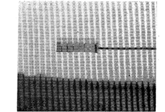
Fig. 4. S t a i n s produced on t h e slide coated w i t h MgO(upper:Obs. No.13, middle:Obs.No.3,lower: Obs. No.?).
Scale : / I
54 Tech. Bull. F a c Agr. K a g a w a Univ. A simple arrangement made of tin plate and steel wire served as a support for glass slide, as shown in Fig. 1. The drift and hence the droplet sizes in it vary with sampling position.. Measurements had to be made, therefore, of the droplet sizes at a fairly large number of sampling points. The collection devices were installed on a pole at eight heights ranging from 30 to 300 cm above ground level. Such four poles with samplers were placed 19 m down-wind from the sprinkler and normal to the direction of the wind, as described
in Fig. 2. As such, the glass slides were
--
arranged in a plane array a t right angle to
.
---
Q @
-
--
.
the wind and the total flux of spray drift past this plane could be determined
CATCH AREA
In the manner in which the drift is caught with coated glass slides, deposition density on them is not independendent of wind ori- entation If care is not taken to place much
emphasis on this fact, a large error would /
'.
.'
--*--.
'
"? POLE EOUIPpED ",.--
--_
_ _ _ - - r r C be caused for estimating the loss due to
WITH SAMPLERS FOR DRIFT
wind drift. Some of the runs were failured Fig 2 Sketch of experimental s i t e due to this cause, but the procedure adopt-
ed did provide the fairly large body of data necessary to yield conclusive answers to the questions posed in this work.
It is very laborious to size and count all the stains found on the slide glass. When the slide is examined a suitable area may be selected to lighten the tedious treatments. Thus, the test must be made of the subsampling procedure to simplify the size-grading.
The evidence for the adequacy of the subsampling
procedure lies in a comparison of counts made on % different spots of the same slide glass by the same 99
~bsever.. Differences between them may include those
caused by inadvertent selective subsampling.. Fig.. 3, go---
-
plotted on the logarithmic probability chart, shows a,
Slide glasscomparison of counts made on three different spots E 70
I
NO 72 of unit area on the same slide. As shown in thisfigure, since the differences between separate sub- samples are small, the error arising from subsampling
seems to be negligible. u o
Thus in our tests the measurement of a droplet
2 1
spectrum of drift consists of three main parts: taking3
'
representative samples of the drift on the plane a o I
L - - - . - c L l
A mrn
reduce the time taken in counting: measurement of
Fig. 3. Evidence for t h e adequacy
the stains in the subsample.. of the subsampling proce-
short distance down-wind outside the sprayed field
By projecting the slides, on which the stains were dure.
r'
1
Vol 15, No 1 (1963) 55 left, onto a frosted glass plate, the stains were enlarged and graded into groups The stains were then sufficiently large to be measured by eye A transparent plate, on which a series of concentric circles were drawn, was placed on the stains projected onto the frosted glass plate for the direct comparison of their areas Thos3e projected stains fitting in-between two concentric circles were taken to have a mean diameter equal to the mean diameter of the two concentric circles
The efficiency of the collecting device is of the greatest importance if a true sample is to be obtained In devices where the drifting droplets impinge on the coated surface, errors may arise due to preferential deposition of the larger droplets and incomplete precipitation of the smaller ones. Accordingly, the correction needed because of the failure of the drift to land on the slide glasses must be madc for low wind velocities when the drift is com- posed mainly of small drops
It is generally known that the "deposition efficiency", i e the proportion of droplets trapped, should be determined by a dimensionless group K=pR2U/18,uW, which is called
the inertia parameter, 1 being the diameter and p the density of the droplet, P the viscosity of the air, W the width of the obstacle and U the velocity of the air. Probably Reynolds
number appropriate to the free stream velocity of the droplet should be included as another parameter An investigation was undertaken by
LANGMUIR-BLODGETT"~)
to determine the rate of deposit of the droplets of different sizes on the front surface of the ribbon type body in a uniform stream of air The curve was obtained showing efficiency of deposition on a ribbon type body as a function of the inertia parameter, K, when the motion of the droplets is governed by Stoke's resistance lawIn a few runs, the drop sizes of the drift and thbe spesd of the wind carrying it werz such that the drift impacted efficiently on these targets. However, a t wind speeds commonly encountered the drift consisted mainly of droplets less than 3 0 0 ~ in size, Therefore, a cor- rection had to be made only for insufficient impaction of smaller droplets, in particular, for low wind speeds near the ground level, using the curve obtained by
LANGMUIR-BLODGETT
for ribbon type body But, as it was thought that for low inertia parameter a correction was not reliable and that thc droplets smaller than 4 0 ~ would cause only a second order error in estimating quantity of drift, the droplets smaller than 40p were not rigorously treatedAtmospheric conditions near the ground
The principle purpose of the present: work is to relate the amount of wind drift to the atmospheric conditions,. Observations will therefore require the meteorological data in the experimental site.
Wind speed mesurements were made with five anemometers which were the sensitive cup type ar~anged to operate electromagnetic counters a t some distance from point of exposme.. They were mounted on a pole a t heights of 35. 65, 105, 155, and 225 cm above ground level with frequent interchanges of instruments. The wind was averaged to the nearest cm per second over periods of approximately five-minutes about each test run. No measure- ment was made of turbulence..
56 Tech. Bull. Fac. Agr. Kagawa Univ. Air temperature and humidity at the 150 cm level were provided by Assmann psychr- ometer.
To investigate the thermal conditions of the atmosphere near the ground, moreover, the temperature differences between two heights of 50 and 150cm were read to O.OZ°C with a thermo-couple on a suitable indicating galvanometer.
The times of observation given in this paper are the mid-points of the 1 to 6 min runs, unless otherwise stated.
Results and Discussions 1 . Wind speed, air temperature and humidity
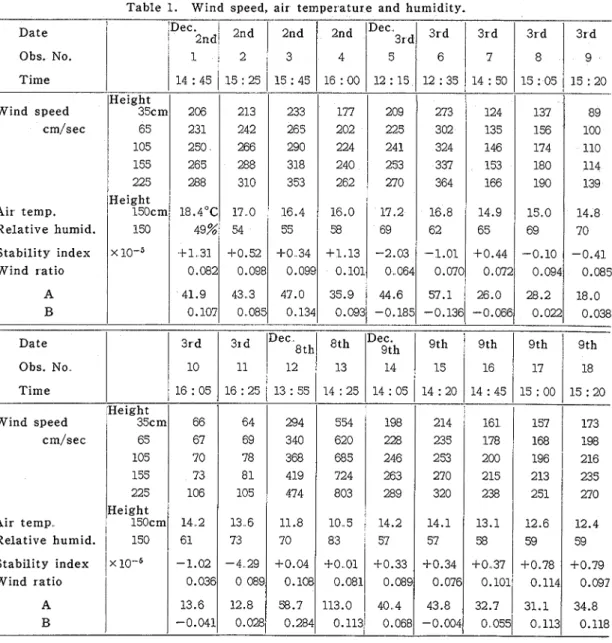
The subsidiary Table 1 contains wind and temperature data in greater detail together with other relevant weather information.
Table 1. Wind speed, air temperature and humidity. Date Obs. NO. Time Wind speed cm/sec Air temp. Relative humid. Stability index Wind ratio A B Date Obs. No Time Wind speed cm/sec Air temp Relative humid. Stability index
I
Height 35cm 65 105 155 225 Height 150cm 150 ~ 1 0 - ~ Height 65 jScm 105 155 225 Height l5Ocm 150 x Wind ratio A B 2nd 4 16:OO Dec. 2nd 1 1 4 : 4 5 206 231 250 265 288 18.4OC 49% t1 31 0.082 41.9 0.107 3rd 10 16 : 05 3rd 5 12:15 0.081 113.0 0.113 0.108 58.7 0.284---
2nd 2 1 5 : 2 5 213 242 266 288 310 1 7 0 54 $0.52 0.098 4 3 3 0085 3rd 11 16 : 25 0.089 4 0 4 0.068 0.036 13.6 -0.041 2nd 3 1 5 : 4 5 233 265 290 318 353 16.4 55 $0 34 0.099 47.0 0.134 DeC 8th 12 13 : 55 3rd 3rd 6 7 12:35 14:50 0.076 43.8 -0.004 177 2 0 9 0 089 12.8 0.028 294 340 368 419 474 11.8 70 $0.04 0.101 32.7 0055/ 202 224 240 262 1 6 0 58 $1.13 0.101 35.9 0.093 0.114 31.1 0 1 1 3 64 67 66I
69 3rd 8 1 5 : 0 5 273 302 324 337 364 16.8 62 -1.01 0.070 57.1 -0.136 9th 15 14 : 20 214 235 253 270 320 14.1 57 $0.34 225 241 253 270 17.2 69 -2.03 0.064 44.6 -0.185 0.097 34.8 0.118 70 73 106 14 2 61 -1.02 3rd 9 1 5 : 2 0 137 156 174 180 190 1 5 0 69 -0.10 0.094 28.2 0.022 124 135 146 153 166 14.9 65 4-0.44 0.072 26.0 -0.066 9th 16 14 : 45 161 178 200 215 238 13.1 58 + 0 37 78 81 105 13 6 73 -4 29 89 100 110 114 139 14.8 70 -0.41 0.085 18.0 0.038 8th 13 14 : 25 554 620 685 724 803 10 5 8 3 $0 01 9th 14 14 : 05 198 228 246 263 289 14.2 57 $0.33 9th/
9th 15 : 00 15 : 20 l7I
168I
198 196 213 251 12.6 59 f 0 . 7 8 216 235 270 12.4 59 f 0 . 7 9Vol. 15, No. 1 (1963) 57 The variation of mean wind speed near a rough boundary surface have been throughly investigated, and a wind profile law of the form
established under neutral conditions U is the mean wind speed a t height z, r the horizontal shearing stress, pa the air density, s an aerodynamical constant of value 0.40 and zo the
roughness parameter of the surface.
Further, there is considerable convergence towards the view that a satisfactory general- ization of Eq. (1) to small and perhaps to moderate degrees of thermal stratification exists in the form of the log-linear profile
U= A In 2/20 -t Bk-zo ) (2)
The time inversion B would characterize the degree of instability on the occasion in question, taking increasing positive or negative value for increasingly stable or unstable stratifications respectively MONIN adn OBUKOV (1954)(1°) have shown further that B should
be given in terms of r and the upward heat flux HI by
B=
-
agH~/rc, Twhere T is absolute temperature and a a universal constant.
There is too much freedom in the direct fitting of Eq. (21, and this may induce highly misleading results. Thus it is preferable that 20 is assigned in advance.
Generally, over the natural sites 20 must be expected to vary with stage of growth, with
wind speed, and possibly with wind direction, However, as the observations were made over the seed field with no parallel ridges and troughs, the roughness may be regarded as con- stant.
No individual profile can be interpreted sufficient to calibrate the site. With present knowledge only neutral conditions can be used for calibration purposes For these reasons a value of 20, the roughness parameter, was obtained by the following procedure.
A wind ratio, R, was defined as follows:
R=C(U4 f U3) - ( U z f Ul):/(U4+Ua f Uz f U I )
where U I , Uz, U3 and U4 are the mean wind speeds a t heights of zl, za, 2 3 and 24,
respectively.
~ r , was Furthermore, a stability ratio, RL', roughly proportional to the Richardson's numb-
defined as follows:
R ~ ' = ( T I ~ o - T ~ o ) / U I O O ~
where T15o and Tso are the mean temperatures
at heights of 150 and 50 cm, and Uloo is the
: O '
[
.
./
mean wind speed a t 100 cm. The neutral con- 2
y ~ ! p o
dition is assumed to occur. when the stability ratio
06 * -o'
is zero. The values of R computed for each run
were plotted against the stability ratio, as shown
,
,,
1.
in Fig 5 The adiabatic value of R, denoted by - 6 - 4 - 2 o 2 - 4 -
Stabll~iy andex X I 0
Raa, was determined from the intersection of this Fig. Variation of wind ratio w i t h
58 Tech.. Bull. Fac. Agr. K a g a w a Univ.. Application of Eq. (1) gives
Raol= (10gzr t 10gza)
-
(10gzz tlogzl) log24 f-10gza f-logzz -I- 10gZ1-410gZofrom which 20 was computed. When =155cm, 23 = 105 cm, zz =65cm and zl =35cm, the values of Raa and zo were 0.087 and 0.27cm, respectively.
Using this value of zo and wind-profile measurements over the site the values of A and
B in Eq.(2) were determined for test runs by methods of regression, as given in Table 1.
As such Eq.. (2) is employed to calculate the interpolated or extrapolated values of wind speeds a t heights where the samplers were mounted.
2. Variation of droplet sizes with height i n drift
The deposit was measured by counting and sizing the drift stains found on sheets of slide glass The stains were enlarged twenty times by a projector and counted in lmm group.. Then, after the corrections for deposition efficiencies, the volume and hence the volume fraction occupied by each size group of droplets were calculated a t each position where the droplets in drift were
sampled. As the larger droplets settle more rapidly than small ones, both the size and number of drop- lets in drift vary with height
At the outset, therefore, analy- ses will be made on how the drift and hence the droplet sizes in it vary with height
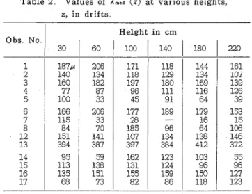
Plotting the cumulative volume percent under size against the drop- let size, the volume median size and the 95 percent size at respec- tive level of height 19m down-wind from the sprinkler were deter mined, as tabulated in Table 2 and 3. In this case the 95 percent sizes were adopted as more suitable, because of consider able experimental errors occurred in determining the largest droplet sizcs a t various heights in drift.
It may be found from Table 2. that the volume median sizes do not remarkably vary with height within the range from 30cm to 220 cm, though the point sscatter wide- ly. Preferably, they seem to be
Table 2. Values of Rmed ( z ) a t various heights,
z, in d r i f t s
Obs No Helght in cm
30
/
601
100/
140/
1801
220Table 3. Values of Rss(z) a t various heights, z, in drifts Height in cm Obs No 30 60
1
1001
1401
180(
220 1 2 3 4 5 6 7 8 12 13 14 15 16 17 288,~ 250 298 207 183 295 174 191 247 552 234 230 321 168 280 244 353 187 149 314 132 168 220 548 316 245 335 193 291 248 339 174 139 331 128 159 240 547 180 265 332 204 268 222 349 221 181 331 205 233 546 300 221 337 205 244 260 342 204 130 326 116 137 274 555 220 223 332 252 270 232 234 223 142 262 104 209 236 539 182 189 272 273Vol. 15, No. 1 (1963) 59 much dependent upon the average wind speed.
To predict the manner in which the 95 percent size a t each level of height in drift varies with the wind speed, we made use of the method of simple physical assumptions, though an exact determination of the trajectories of the droplets would, of course, be very corn plex.
Let x represent distance in the horizontal down-wind direction, and h vertical distance (as depth, increasing downwards). The coarse droplet continues its original trajectory but the small droplet loses its momentum and is slowed rapidly to the air velocity. Accordingly, assume that a drifting droplet moves together with an air stream from the starting position; i. e., dx/dt= U(h), where U is the wind speed in the x direction, and let the rate of descent of the drifting droplet be a function of depth; i. e., dh/dt=v(h).
Then for the trajectory of the droplet,
dx/dh= UCh)/v(h), (3)
and the equation of the trajectory can be stated as
in which .xo is the horizontal distance of formation of the droplet.
For droplets of the size with which we are concerned, evaporation in flight is considered to be low, possibly negligible in the time taken. By assuming that the rate of descent of the droplet is always equal to the terminal velocity, v,, Eq.(4a) is rewritten as
The velocity of the wind is not independent of height. In particular, at ground level, the air velocity is small, so that a drifting droplet which reaches that level is, unless it evapo- rates, very likely to settle a t a steep angle.
Therefore, substitution of a wind profile law, Eq. (21, in Eq. (4b) gives h
X -
xO=L
V,1
o { ~ ~ n H ~ h + ~ ( ~ o - h-z0))dh ( 4 ~ 3in which z=Ho-h
..
Ho is the height above the ground level of formation of the drifting droplet, and z= Ho for h = 0 .Setting
Eq. (4c) may be written in the nondimensional from
g(x--.x,)/~av,=gh/v,2 (6)
where
Ga
is the average wind speed throughout the depth from 0 to h, i.e., throughout the height from z to Ho.In general, the terminal velocity, v,, is given by the following relationship:
where CD, the drag coefficient of the sphere, is a function of the Reynolds number
Re=
v,A/v, and pa and Y are the density and kinematic viscosity of the air:It has been shown experimentally that drops of various liquids falling through air are deformed to a negligible extent provided that the value of pA2g/o is below 0.4. In this
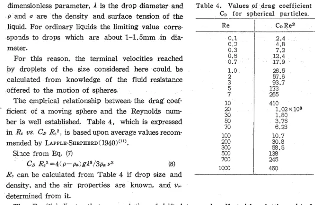
60 Tech. Bull, Fac. Agr. Kagawa Univ. dimensionless parameter, R is the drop diameter and
p and a are the density and surface tension of the liquid. For ordinary liquids the limiting value corre- sponds to drops which are about 1-1.5mm in dia- meter.
For this reason, the terminal velocities reached by droplets of the size considered here could be calculated from knowledge of the fluid resistance offered to the motion of spheres.
The empirical relationship between the drag coef- ficient of a moving sphere and the Reynolds num- ber is well established. Table 4, which is expressed in Re US CD Re2, is based upon average values recom- mended by
LAPPLE.~HEPHERD(~~~~)('~).
Sizce from Eq. (7)
CD Re2=4(0-pa)gRa/3pa v 2 (8)
Re can be calculated from Table 4 if drop size and
Table 4. Values of drag coefficient CD for spherical particles --
Re
I
C D R ~ '0.1
1
2.40 2 4.8
density, and the air properties are known, and v, determined from it.
Thus Eq. (6) indicates that a correlation of drift data can be effected by plotting gh/vm2 against g( x- xo)/Ua V-..
It may be supposed that the largest droplets a t various heights in drift are formed near the maximum height to which the water jet issuing down the wind from large orifice rises. At an operating pressure of 2.5 kg/cm2, the water jet from large orifice rises to the height of about 4m a t the distance of about 9m from the sprinkler. Then x-x0=1000cm and h = (400-z)cm are substituted in Eq. (6).
Using the 95 percent sizes obtained a t eight heights of 30, 60, 100, 140, 180, 220, 260, and 300cm above the ground level, g(x-xo)/ua V, was plotted against gh/vm2 in Fig 6, where ex- perimental and theoretical data were compared.. The points from our data scatters widely, but fall close to the theoretical line. As such, we know that Eq.. (6) provides a conveniently con- cise expression which is sufficiently close to the experimental results for practical purposes. Fig. 6 indicates that the drift contains larger droplets near the ground and that the 95 per- cent size a t each level of height in drift in-
creases with wizd speed, as expected upon con- g(x-xO) / f l u ,
sideration of Eq. (6). Fig 6 . Variation of Rss(z) with height in drift.
Vol. 15, No. 1 (1963)
Obs No 8
Droplet diameter mm m )II
Ohs No 4
Average wind speed
. ,*
.
244 cm/ sec0 0 1 0 2 0 3 0 4 0 5
Llroplcr dlamctcr mm Obs No 15
Average wind speed 275 crn/sec
Obs No 2
Average wind speed 290 c m / s c c
0 , ' . . , .
.
, 3 7 3 . .0 0 1 0 2 0 3 0 4 0 5
Droplct diameter "'"I
'
O
Average wind speedt
r
N
a
333 cm/ sec Droplet diameter mm
1
Obs No 12 1 Average a i d ~ p r c d 426 c m / sec Ohs No 13 Avcl agc ~ i l l d spced735 c m / scc
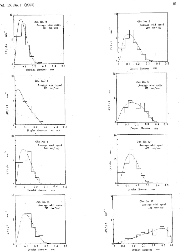
Fig. 7. Frequency d i s t r i b u t i o n s p l o t t e d b y increments a n d Upper Limit frequency c u r v e s on volume basis, of d r i f t s u n d e r various wind speeds.
Tech.. Bull.. F a c . Agr. K a g a w a Univ. 3,. Spectrum and mean szze of d r t f t It is of practical value to know the spectrum and mean size of the total drift which is carried off by the wind.
Using the data concerning the number of droplets occupied by each size group a t each sampling point, the total number and hence the total volume of droplets occupied by each size group in the total flux of drift past a vertical plane outside the sprinkled field were easily determined, as given in Table 5.. In Fig. 7 the volume fractions divided by the size interval, that is, the volume frequen- cies, AV/Al, are plotted against each mean of size group.. A comparison between these results shows that a coarser drift arises a t higher wind velocities, as would be expected..
Many attempts have hem made to fit distributions of droplet sizes with empirical mathematical formula.. One such formula, introduced by MUGELE and EVANS"", is likely to fit the data better than equations previously used
and is of the from
.Y
being defined byal y = In-
Am,- R
where dV is the volume fraction of droplets with diameters in the range
In this case, the size distribution of droplets in the drift will be complete- ly characterized by (1) the upper
limit size Rm, (2) the size parameter a,
Vol 15, No. 1 (1963) 63 As such, the cumulative volume fraction of drift smaller than stated size was plotted against I / ( Am-- 1) on logar ithmic-normal probability paper. Fig. 8 shows typical spectra of
No 2 290 cm/ sec 0 No 8 182 @ No 13 735 0 I
I
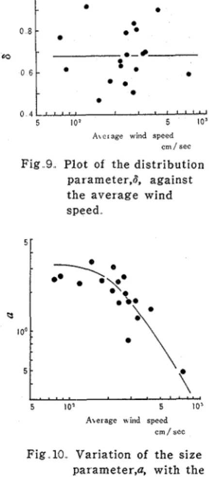
lo--' 5 loo' 5 10' / ( A m - A ) F i g 8 Upper-Limit % 99 9 99 90 70 50 30 10 B No 6 333 cm/ sec A / ( A m - A ) analysis of datadrift.. These data are all believed to fit the straight l i n e within the accuracy of method and measurement. It is apparent, therefore, that Eq. (9) provides an effective means of correlating the data obtained in our cas,z.. The size-distribution curves of drifts correlated by the upper limit equation were superimposed in Fig.. 7. The values of a and 6 were determined for each test run in the way described in Ref. 1, and presented in Table 6.
T a b l e 6. Size-distribution and mean size of droplets in drift and percentage of s p r a y drifting initially
Q : Quantity of drift. QO : Quantity of initial drift..
64 T e c h . Bull. F a c Agr. Kagawa Univ In such works the volume median diameter is often quoted; this is the diameter about which the volume is equally distributed, and determinable from the line representing the distribution
Probably a better parameter, and one which is often quoted in allied field of research, is the Sauter mean diameter This is the diameter of a d~oplet that has the same ratio of surface area to volume as the entire spectrum of droplets. Its value is most affected by the droplets of intermediate size, and its use therefore tends to minimize the effect of inaccurate measurements a t both ends of the spectrum, where errors are greatest. The Satuer mean diam?ter, A,,, has been calculated indirectly by the relationship derived from Eq (9) (see Ref 3).
Table 6 summarizes the mean diameters for eighteen different runs
The eventual drift leaving the sprinkled field after portion of it has settled to the ground is dependent upon the particular circumstances However, it seems difficult if not impossible that a detailed mathematical and physical description is made of the process of drifting by the wind as water is emitted from a sprinkler head. I t is the wind which determines whether or not the small droplets are winnowed out of the spray, for which reason correlation of drift data obtained from the experiments with wind data would be of some value, even if not exact In our case, the problem I O -
corsists in correlating a, 6 ahd Rm, respectively, with
wind data 0 8 -
Fig 9 shows the plot of the distribution parameter, 6,
-
0 6 -
agairst the average wind speed. The random scatter of the data indicates that the distribution parameter would
.
• •
-
0-0-t
.
.
.
not be dependent upon the wind speed, which results o 4 f ' a ' *
i s ,
5 lo1 5 l o 3
in a horizontal line on Fig. 9, A\ c r age wmd speed
cm / sec
Fig 10 shows the variation of the size parameter, a, Fig 9 Plot of the distribution with wind speed From this figure it is seen that an parameter,$, against increase in wind speed will decrease the size parameter. the average wind
speed AS stated, determination of the upper limit size is
clearly subject to experimental error. Instead of it, therefore, we used the 95 percent size as a more suita-
ble for correlation of data with wind conditions. It may
**$
be supposed that the formation of the 95 percent size 0.droplet in drift occurred near the highest position to which the water jet from large orifice rose when issued down the wind Accordingly, on the basis of such pre-
5
QL
3 m . . m.\
sumptio~s as previously mentioned, the 95 percent size in
drift was correlated with the average wind speed in the 5 l o =
1,
,
5 10'
way described in Section (2) of this report A ~ e r a g e ntnd speed crn / sec In this case, the relationship is written in the form
00) Fig
10 Variation of t h e size
gL/Ux V, = g H O / v w 2
parameter,a, with the in which
L=
x- x , = 1000cm,Ho
= 4OOcm, and V- presents average wind speedNol. 15. No. 1 0963) 65
Fig. 11. Variation of gH,/v-'
.,
with gL/Uxvoo.5 r
--L
-5 lo2 5 10'
Average wind speed
crn/ree
Fig.12. Effects of wind speed on volume median size of drift.
Average wind speed cm / sec Fig. 13. Effects of wind speed on
Sauter mean size of drift.
the terminal velocity ... corresponding to the 95 percent size drop in drift. Utr is the average wind spa2d thoughout the height considered here (from zo to Ho)
and calculated by
Fig. 17 shows the comparison of experimental data
-
with theory for the variation of gL/Ux V- withgHo/vm2. There is a remarkable agreement between
con- the theory and the results obtained. It may b,
cluded from this figure that an increase in wicd s p e d increases the 95 percent size, nearly corresponding to the maximum droplet in drift, which is to be expect- ed upon consideration of Eq. (10).
The volume median drop size and "he Sauter mean drop size of the drift a t an operatbq pressure of 2.5 kg/cm2 and at various wind speeds are shown in Fig. 12 and 13. The increase in wind speed is thus seen to lead to larger droplets. For example, a t 3 and 7 m/sec the volume median diameters of drift were 135 and 315 ,a,
respectively.
Finally, there remains only for consideration how much drift would occur in particular cir- cumstances. The total flux of drift past the test plane was deter- mined. This total drift was noted as a parti- cular fraction of the sp ray which gives rise to it, and is shown in Fig. 14. The amount of drift at 19 m was of the
order of one-hundredth
0 1
of the amount of the
5 ! ' ' ' l i z
5 ' " "~10'Aver age a i n d speed
whole spray from the cm/ see
two-nozzle sprinkler Fig 14 Effects of wind speed and increased in propor- on percentage of spray
66 T e c h Bull. Fac. Agr. Kagawa Univ. of the average wind velocity. At wind speeds of 3 and 7 m/sec, the quantities of drift were 0.4 and 5.2 percent, respectively.
4 . Percentage of spray drZfting i n i t i a l l y
It is necessary that the above-obtained results are inverted to obtain a measure of the percentage of sprays drifting initially, for drifting droplets evaporate in the journey.
A series of tests was made in late fall when the air temperature was considerably low.
It was reasoned that the evaporation in this season would be low, possibly negligible. However, droplets in drift are so small that some allowance for evaporation has to be made before the quantity of spray drifting initially is estimated.
Although a large number of articlm have been published on the quasistationary evapo- ration of drops in a stream of gas, i. e., of drops moving relative to the medium, they seems to be too complex to be used in our works.
It is the simplest case of evaporation where the drop is motionless relative to the medium and the hydrodynamical factor is absent. Although, strictly speaking, this never occurs in practice, the motion of droplets, if sufficiently small, does not affect the rate of evaporation and therefore the theoretical or experimental results on quasistationary evapo- ration of droplets motionless relative to the medium remains true for such droplets.
For these reasons, corrections for evaporation of droplets in our tests on wind drift were
ing devices is approximately equal to the distance Arerage wind speed
made using the relationship obtained in the previous paper");
-
c m / scc
between sprinkler and sampling device devided by
Fig 15 Effects of wind speed on the the average air speed; t = ~ , / & where Lo the percentage of s p r a y drifting
AO2--A2 =ZC( 1 - H , t
Q
in which A0 is the initial diameter of droplet, t the
10'
time in flight, lOOH the relative humidity and C
given in Table 3 in Ref. 1. 5
3
It is very difficult or impossible, however, to d e
,
0
termine with accuracy the time taken in flight from
a
production to deposition for each droplet in drift.
l o o . Sprinkler head rotates slowly to distribute water
$
uniformly in all directions and the small droplets 5 'E which become drift lose their momentum in a very % short time to move with an air stream. It may be "
5
supposed, therefore, that on an average the droplets g
;
l o - 'in drift would have been produced originally over c
the sprinkler head. Furthermore, it is permissible to 5
consider the drifting droplets moving with an air stream from the start.
It follows from these presumptions that the time taken in flight for droplets depositing on the sampl-
distance between sprinkler and sampling device initially.
/
' 5 " ' ; 0 2 -I
,--• * a a a/ a* •p
' " 5 " " l o 3Vol. 15, No. 1 (196'3) 67 (=1900cm) and
3~
the average air velocity.Fig. 15, in which the effect of wind speed on percentage of spray difting initially is plotted, shows the approximately ten-fold increase in quantity of initial drift with a change of wind speed from 3 to 7 m/sec At a wind speed of 7 m/sec, the initial drift increased to 10 percent. The increase in wind speed is thus seen to lead to higher percentage of spray drifting initially.
A comparison could be made between two results obtained from measurement of sprays depositing on a plane array of glass plates and indirectly from measurement of precipi- tations on the sprinkled area
In previous work''), a test plot was set up for collecting the discharge from the same sprinkler equipped with 3/16 x 1/8-in nozzles by arranging cans on the ground a t 3m spacings. About 21 tets of one hour duration at an opwating pressure of 2.5kg/cm2 were run under various wind conditions, at cloudy weather in late fall The loss from spray has been commonly noted as the difference between the discharge and the computed amount of water reaching the ground surface, corrwted for the evaporation losses which occur after the water reaches the gage cans.
The curve (A) of Fig. 16 shows the results of spray losses obtained when the correction factor is applied to the evaporation loss3es from ths gage cans. It is s.ecn from this curve that losses as low as 4 percent may be expected at low vapor pressure deficits and with nearly zero wind movement, and that comparable losses a t a wind speed of 5 m/sec may run up to 11 percent
The shaded area in Fig. 16 indicates the percentage of spray drifting initially. A comparison between these two 20
results shows that considerable
quantities of initial drift expected 1 5
from measurements of the total spray losses were not found on
-
10targets 19m down-wind. It must be 5
*
remembered that in this report " 5
drift is arbitrarily defined as the
quantity of spray reaching targets o
0 I 2 3 4 5 6 7
19 m down-wind. A k ~ ~ a g r KIN^ S P C C ~ ~ I / ~ C L
Accordingly, the discrepancies Fig.16 A comparison between s p r a y l o s s e s obtained are accounted for partly by the f r o m t h e can t e s t s a n d quantities of initial
d r i f t fact that the record was obtained
about 19 m down-wind from the sprinkler, for which reason considerable quantities of
fine spray had settled onto the ground before reaching the targets It is evident that much of the fine spray was carried out of the catch area but that considerable quantities of it, which could not be measured by the gage cans, settled in the outer fringe area up to the targets. The wind controls this rate of fallout of fine spray onto the ground outside of the can area Spray losses determined from the can tests are probably those due to (1) settling of droplets in the outer fringe area (outside of the catch area up to the targets), (2)
68 T e c h . BulI. Fac. Agr.. K a g a w a Univ.
evaporation from droplets before reaching the ground (the catch area and outer fringe area), (3) complete evaporation in the air of fine mist, for which reason it fails to reach both the ground and the target and (4) wind drift, corrected for the evaporation in the journey.
The quantity of fine mist that fails to reach the ground and also the target, owing to complete evaporation in the air, will be roughly estimated by using the expression for the evaporation of a water droplet and the size distribution function of sprays emitted from the sprinkler nozzle.
I t may be considered that such fine mist was formed near the sprinkler head. Then, a limiting drop size such that all smaller droplets evaporate completely in the air can be determined under a specified condition. Of course, there is not such a clear-cut upper limit to the drop size, so that the following method gives only a rough approximation.
At first a drop size such that all smaller droplets evaporate completely in the time taken to travel from near the sprinkler nozzle to the target will be estimated by considering a fine droplet moving together with an air stream.
By putting ~ = L O / ~ I Z (the time required for complete evaporation) and A = 0 in Eq.
0,
wehave
A% =BC(I - H ) L ~ / & Q
Secondly, the size of drop that fails to reach the ground owing to complete evaporation will be determined. Suppose that such a fine droplet is falling throughout at terminal veloc- ity. For the terminal velocity in air of droplets of the size encountered in our case, it is convenient to use an empirical equation
A
v. = A' i 2
ex^(-^)
a4in which A'=30.2 x 104cm-I sec-I and B=O.O433cm, at 15°C air temperature. Units of v,
and A in Eq.04 are cm sec-l and cm, respectively.
Let h be the vertical displacement (as depth, increasing downwards) and let v.. be the
terminal velocity a t time t .Here the rate of descent of the droplet dh/dt is equal to v,. Accordingly, using Eq. Q and 04, we have the equation
A A
d h / d ~ = - - ~ / i 2 e x p ( p p )
C(1-H) (15)
Eq. (15) can be rewritten in terms of a dimensionless vertical distance F=BC(l-H) h/v-o A$
and a dimensionless diameter D=A/Ao; namely
d ~ = -2Da e x p ( b ( 1 - D ) } ~ D (Is)
Thus by integrating Eq. (1Q between the limits D = 1 , D = D, and F= 0 , F= F, we are led to the following solution:
B' 2
F = ~ ( E ) [ { D ' + ~ D ~ ( $ ) + ~ D ( ~ ) o + 6 ( $ ) a ) e r p { ~ ( l - ~ ~ }
Eq. (17) gives us the displacement as a function of D . Now putting D= 0 in Eq. (171, the
vertical distance the droplet travels until it has completely evaporated is written in the non-dimentional form
Vol 15. No. 1 (1963) 69
As such, using Eq 43) and
(a,
we can determine a limiting drop size such that all smaller droplets fail to reach the ground and also thc targetSuppose that h(R= 0 =100cm or soCnearly equal to the height of the sprinkler riser-pipe)
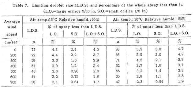
and Lo = 1900cm Then the limiting sizes a t 60 percent relative humidity and 15°C air temperature are calculated for stated wind speeds, as shown in Table 7
.
Consequently, the fraction of spray less than the limiting droplet size would be determinable in the following manner by reference to the complete drop spectra of the spray produced by the sprinkler.Table 7. Limiting droplet size (L D S) and percentage of the whole s p r a y l e s s than it. (L O.=large or ifice 3/16 in, S 0 =small or ifice 1/8 in)
If we use the upper limit equation for describing droplet size distributions in sprays emitted from a sprinkler nozzle (See Ref. 31, the cumulative volume fraction of droplets with sizes smaller than the limiting size 20 will be evaluated by
Average wind speed
yo being defined by
At 2 5kg/cm2, 6 is 0 404 or 0 519, R o , 4 24 or 2 95 and a 2 85 o r 2 50 for large o r small orifice, respectively. Now we obtain the percentage of thee whole spray from the two-nozzle sprinkler evaporated completely under a specified condition, as seen in Table 7.
Of course, if formed a t higher levels, larger droplets wauld fail to reach the ground. This fact would probably lead to an underestimation of loss du3 to complete evaporation of fine mist No quantitative evidence is as yet available to show where fine mist is produced as the jet is ejected from a nozzle It is true, however, from actual observation that much of the fine mist considered here was produced near the sprinkler nozzle Consequently, the computed values are now available as an approximation for purposes of comparison, as shown by the curve ( B ) of Fig 16.
In Fig. 16, zones (
I
) andC I I )
illustrate losses due to complete evaporation and wind Air temp :15OC Relative humid :60%% of s p r a y l e s s than L D.S L D S
1
L O
I
S O .I L O ~ S O .
Air t e m p : 30°C Relative humid.: 50% % of s p r a y less than L D S. L D S
1
L.0. S OILO.+S.O.
c m / s e c i i c %j
% %1
i l l %I
%I
% 4.7 4.7 3.8 3.1 2.7 2.3 1 9 3 0 3.0 2 1 1.6 1 4 1.1 0 94 0 200 300 400 500 600 700 86 86 7 1 62 55 50 47 5.5 5 5 4 5 3.7 3 2 2.8 2.3 77 72 59 51 45 41 38 4.8 4 4 3,5 2.9 2.4 2.2 1.5 1.2 0.90 4 0 3 7 2.9 2.4 2 02
1
0 75 2.1 0 64 - -1.8 1.770 Tech. Bull. Fac. Agr. Kagawa Univ. drift, respectively. Accordingly, the remaining zone
(1
) could be probabIy ascribed in large part to settling of droplets in the outer fringe area and in small part to evaporation in flight from considerably large droplets before reaching the ground (the catch area and outer fringe area). The former, which occupied a great part of zone(I
I, was considerably higher at the high wind velocities, but did not moisten the soil in measurable quantities outside the catch area, for which reason it was thought that it would be a loss. However, as this loss is actually due to evaporation which occurred after the droplets had reached the ground surface outside the catch area, there is some objection to looking upon it as part of spray losses.In the can tests, from which spray losses were calculated, only a single sprinkler had been operated. It is natural, however, that spray losses should be always evaluated under field conditions with overlapping spray from adjacent sprinklers. In the tests in which two s~rinklers were operated, FROST and SCHWALEN computed the spray losses on the basis of the overlapping area between the two sprinklers and verified that the losses were greatly reduced. We may clearly say from such a viewpoint that the amount of water falling onto the outer fringe area is not nec~sarily a loss, even though it is not enough to moisten the soil in operating a single sprinkler alone.
Consequently, in the sprinkler method of irrigation, losses due to wind drift does not occur to a detectable extent a t mod2rata wind s p ~ d s . Such spray losses determin'ed from the can tests, which have been widely used for practical purposes, lead to improper low efficiency in sprinkler irrigation
Acknowledgment
T h e author's thanks a r e due to Messrs. K. FUMOIO, T NAGAO, and I YOSHII for their assistance in carrying out the experiments The help of Miss. N. KITAHAMA in making t h e calculations and charts is gratefully acknowledged
References (1) INOUE, H , JAYASINGHE, S S : Tech Bult. Fac.
A g r Kagawa Univ , 13, 202 (1962).
(2)
-
: Reports for Discussion, Question 16, R7. 5th Congress I C . I . D., Tokyo-1963.
(3)
-
: Tech. Bull. Fac Agr Kagawa Univ ,14, 160(1963).
(4) CHRISTIANSEN, J.E. : California Agr. Exp. Sta ,
Bull. 670, October-1942
(5) FROST, K. R, SCHWALEN, H C : Agricultural Engineering 36, 526(1955),
(6) SHIRAI, K. : cited in Hatachi-Kangai (Field-
Irrigation), edited by YAMAZAKI, F., HASEGAWA, S .161(1959), Tokyo, Nosangyosonbunka-Kyokai (in Japanese).
(7) SUGI. J , INOUE, H. : Tochikairyo, 11, 93 (1961)
(in Japanese)
(8) MARUYAMA, M , HAMA, K : J. Met. Soc. Japan,
Ser. 1, 32, 6(1954)
(9) HUAN MEI-YUAN : Izv. Akad. Nauk. S. S. S . R., Ser. Geofiz., (10) (1962)
(10) MONIN, A. S., OBUKOV, A. M : cited b y YAMAMOTO, G , J. Met. Soc. Japan, Ser. 1, 37,
60(1959).
(a
LAPPLE, C. E, SHEPHERD, C. B. : Ind. EngChan , 32, 605(1940).
(12) LANGMUIR, I., BLODGETT, K. B. : cited in Che- mical Engineers' Hmdbook, 3rd Edition, edited
by PERRY, J.H.,1022(1954). New-York, McGraw- Hill
(13) MUGELE, R A , EVANS, H.D. : Ind. Eng.'chem , 43, 1317(1951).
Vol.. 15, No. 1 (1963) 71
33 E @%%--x 7-11 ~ ? & l 2 M L f i can test ~r~¶@&%i%z4W#%&R%7ri $ 7 ~ ; ~ k i E T i b , %!kt 2$2 brj;k % a % , ?OfIvk 9 039fI>%-x 7'9 Y P 7 -O$k7kfi$OFI2h.< tzP$7S(?6 %RB%Tbb, %WO
R911 . / ? ? - & ~ Z ~ L X f i ~ A @ L \ T 6 O T & l j f I ~ b , &-37"11 Y P ~ - O % & ~ % O F I ~ ~ < ~ ~ P $ ~ ~ ' ~ ~ ~ % O % # % ~ J L I " ~ T o ~ ~ , j p i 3 ~ 7 " s ~ . zt11 Y P 5 - 0 ~ 7 i ( g f i + F ~ J R - F K , M ~ O - C L \ S L ~ C ~ ~ ~ F&%BZF@K
RZB
L T , %%H%%B$2@laL-c c h t ~ g ~ . 7 ,fFt%-f
6 @$R7k%%0$3@9&, 'FLS@,&A@&,
SkLSAzAB? - 8 tr$BHLfc S;.fXB%B%Ck, gF%ii=/J\s