Panel Data Research Center at Keio University
DISCUSSION PAPER SERIES
DP2015-006 December, 2015
Intensive and Extensive Margins of Japanese Male and Female Workers - Evidence from the Tax Policy Reform in Japan-
Yusuke Inoue*
【Abstract】
Using the annual micro panel data of Keio Household Panel Survey, I estimated labor supply models to identify the intensive and extensive margins of Japanese male and female workers. My empirical results contradict earlier studies which finds large intensive margin of male workers. The findings are while, for all male workers, hours worked elasticity and labor force participation elasticity are quite small (0.009 and 0.0025 respectively), extensive margin of non-regular workers shows big sensitive response (0.365). On the other hand, intensive margins of both workers are small against wage changes. The investigation by separating age groups (over 55 and under 54) shows that the sensitive labor participation response is caused by elderly non-regular male workers. Furthermore, the comparison between male and female labor supply responses ensure that both margins of male are much smaller than those of females. The result also reveal interesting feature of female work behavior that the intensive margin of female regular workers is as small as that of male.
Keywords: Taxes, Japanese Male Labor Supply, Lifecycle-Consistent Fixed Effects model, Selection, and Endogeneity
*
Deputy Director in the Japanese Ministry of Health, Labour and Welfare
Panel Data Research Center at Keio University Keio University
1
Intensive and Extensive Margins of Japanese Male and Female Workers
- Evidence from the Tax Policy Reform in Japan-
Yusuke Inoue1
Abstract
Using the annual micro panel data of Keio Household Panel Survey, I estimated labor supply models to identify the intensive and extensive margins of Japanese male and female workers. My empirical results contradict earlier studies which finds large intensive margin of male workers. The findings are while, for all male workers, hours worked elasticity and labor force participation elasticity are quite small (0.009 and 0.0025 respectively), extensive margin of non-regular workers shows big sensitive response (0.365). On the other hand, intensive margins of both workers are small against wage changes. The investigation by separating age groups (over 55 and under 54) shows that the sensitive labor participation response is caused by elderly non-regular male workers. Furthermore, the comparison between male and female labor supply responses ensure that both margins of male are much smaller than those of females. The result also reveal interesting feature of female work behavior that the intensive margin of female regular workers is as small as that of male.
Keywords: Taxes, Japanese Male Labor Supply, Lifecycle-Consistent Fixed Effects model, Selection, and Endogeneity
1 Deputy Director in the Japanese Ministry of Health, Labour and Welfare.
2 1. Introduction
Estimating the effect of income taxes on the labor supply has been a centerpiece in labor economics researches over decades since labor supply elasticity estimation is essential for the calculation of social welfare loss caused by public policy. However, compared to works in U.S. and European countries, relatively small portions of researches have addressed to identify labor supply elasticity in Japan. Especially, there are few results regarding the labor supply responses of males who play a core role in the Japanese labor market.
The main purpose of this paper is providing new evidence in the Japanese male labor supply responses based on the lifecycle consistent structural model with recently developed micro-panel data, exploiting tax policy changes in 2006 and 2007 to deal with potential endogeneity problem. Also, to check and compare the validity of empirical specification used in this paper, I similarly estimate female labor supply responses since those studies have been more accumulated than males. Besides, to respond growing concerns on the Japanese labor market in which non-regular workers have been increasing, I estimate two separate labor supply responses for non-regular and regular workers for males.
Although bunch of literatures try to capture labor supply elasticity, there is no consensus on how exactly male and female response against tax and wage changes. Keane (2011) surveys existed labor supply literatures and finds that uncompensated wage elasticity for males are ranged between 0.47 and 0.7, and its average is 0.04, while the elasticity for female is between -0.2 and 0.89, and its average is -0.292. Bargain, et al. (2012) take a large-scale international comparison of labor supply elasticities. Their survey shows that the wage elasticities across countries are relatively small for both sexes, but the labor force participation elasticities are
3
bigger than the wage elasticities. Also, there is a view that male workers show relatively small labor supply elasticities compared to female workers.
On the other hand, although there are empirical analyses for elderly and female labor supply in Japan, as far as I know, there are few articles investigating male labor supply issue. Asano (1997) estimates the price elasticity of goods by Almost Ideal Demand System (AIDS) with pooled-aggregated data of 47 prefectures. In this research, he finds compensated wage elasticity is 0.39. Yamada, et al. (1999) employ AIDS method to estimate labor supply of men aged 25-39 with aggregated data on prefecture basis. His estimation also indicates relatively big wage elasticity (0.37). Kuroda and Yamamoto (2008 (a)) establish aggregated data by prefecture, age and sex to estimate Frish elasticity with life-cycle consistent labor supply model. Their estimates of intensive margin for male workers are in a range of 0.14 to 0.24.3
However, although Japanese economists find relatively large value of intensive margin among male workers compared to findings in other countries, more accurate estimation should be required utilizing micro data. In my best knowledge, only work so far estimating male labor supply responses with consideration of personal income tax using micro data is Bessho and Hayashi (2005), and their sequential work of Bessho and Hayashi (2011). Their 2011 paper tries three ML methods with the largest cross-sectional labor survey of Japan (Shugyo Kozo Kihon
Chosa) focusing on the prime-age male aged 25 to 55. While their estimates show large
variations of values of intensive margin, they conclude that their findings are still bigger4 than those estimated in other countries’ studies.
3 Their research (2008 (b)) is one of the most related works of this paper. They try to estimate the wage elasticities
of two different employment types of female workers by the similar method used here. However, the paper does not consider the presence of income tax.
4 Three models used in the paper show the average of uncompensated elasticity for single-earner-male with
4
As we have seen above, there are scant amount of literatures regarding estimates of Japanese male labor supply, and only Bessho and Hayashi estimates the labor supply response considering the tax system with cross-sectional micro data. However, surprisingly, there are no attempts to estimate male labor supply in Japan with micro-panel data. The simple reason may be that there had not been available micro panel data which contains necessary information of males, although relatively long panel data has been existed for females in Japan. Thus, this paper exploits
recently developed Keio Household Panel Survey (KHPS), which is the first comprehensive survey to respond such a demand, and has been implemented annually since 2004.
The empirical strategy used here tackles the simultaneity problem of working hours and after-tax wages utilizing Japanese personal income after-tax reforms implemented in 2006 and 2007. Since the tax reform which is not implemented considering change of each individual’s working hours could generate exogenous variation in after-tax wage, the reforms are typically thought to provide ideal natural experiments. The empirical method also considers other well-known problems (Selection bias and division bias) which hamper researchers to get the consistent estimators.
The contributions of this paper are the first to estimate lifecycle-consistent labor supply elasticities of Japanese males and females with micro-panel data, taking into account the presence of nonlinear taxation with a two-stage budgeting framework following the method of Kimmel and Kniesner (1998), and Ziliak and Kniesner (1999). Secondary, the paper
distinguishes different labor responses of non-regular and regular workers, considering
multinomial labor participation decisions with the correction methods of Dubin and McFadden (1980), and Semykina and Wooldridge (2010).
5
My empirical results contradict earlier studies which finds large intensive margin of male workers. The findings are while, for all male workers, hours worked elasticity and labor force participation elasticity are quite small (0.009 and 0.0025 respectively), extensive margin of non-regular workers shows big sensitive response (0.365). On the other hand, intensive margins of both workers are small against wage changes. The investigation by separating age groups (over 55 and under 54) shows that the sensitive labor participation response is caused by elderly non-regular male workers. Furthermore, the comparison between male and female labor supply responses ensure that both margins of male are much smaller than those of females. The result also reveal interesting feature of female work behavior that the intensive margin of female regular workers is as small as that of male.
The paper is organized as follows. The next section presents brief explanation of Japanese labor market and tax policy. The section 3 describes theoretical background of labor supply with non-linear tax system and empirical strategies. The section 4 explains about the dataset and key variables’ data construction. In the section 5, the results are discussed. Finally, I will make conclusions from the obtained results.
2.1 Japanese labor market
Traditionally, core workers of Japanese labor market consist of male regular workers who are typically considered as permanent contract workers until mandatory retirement. However, proportions of non-regular workers, who consist of fixed-term contract workers, dispatched workers and part-time workers, have been growing in all cohorts. As table1 shows, proportions of non-regular workers are rapidly increasing from 1995 especially in younger cohorts. Initial surge for all cohorts had been caused by the long depression after housing bubble exploded. At
6
that time, firms suffering from increasing debt had started to adjust employment and decrease wage level. This effect has disproportional effect among workers. Genda (2001) highlights that the cost of the long recession in Japanese economy was born disproportionately by young people because cutting new hiring is much easier than firing incumbent workers. The white paper of labor economy by Japanese Ministry of Health, Labor and Welfare (2012) also points out that reasons why this trend still continues are : 1) firms are willing to save labor cost and respond business cycle more flexibly, 2) workers tend to choose comfortable working time for their life style.
It is worthwhile mentioning types of non-regular workers to introduce their working patterns. In this paper, non-regular workers consists of part-timers, fixed-term contract workers(Keiyaku
Shain), fixed-term contract after retiring (Syokutaku), and dispatched workers. Part-timers
account for the largest portion of Japanese non-regular workers. They are defined as those who work shorter than other regular workers in workplaces. The Keiyaku Shain is the person whose work contract is not permanent and limited for several years, while they work full time.
Syokutaku is a subset of Keiyaku Shain. But, they are employees who have reached mandatory
retirement age and are rehired under temporary working status. Dispatched workers are persons who are dispatched from their employer to user-companies. Of all those workers, Syokutaku would show quite different working patterns because they basically got the retirement benefits, so, unlike younger non-regular workers, they are considered to work in a more flexibly way. Thus, when we estimate labor supply, we need to be careful about their existence.
This increasing number of non-regular workers has caused political concerns because their salaries level is lower and employment protection is weaker than regular workers, which could
7
cause fears of a future expansion of poverty and an increasing burden of social security. In an economics sense, it is also important to identify their behavioral features against wage changes.
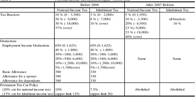
2.2 Tax policy reform in Japan
In this section, I will explain about Japanese tax policy, especially for personal income taxes and its recent reforms which are considered in the analysis. Earning of employed workers in Japan is withheld by personal income tax system which is classified as two components; national income tax withheld by national government and inhabitant tax withheld by local government. Combined income tax brackets are progressive, ranging from 10% to 50% corresponding to taxable income levels. The recent tax reform in which tax brackets were changed is the 2007 tax reform. One of objectives of this reform is transforming the fiscal resource from the national government to local governments without putting additional income tax burden to people. Thus, even though tax brackets for each tax system have been reformed, its combined average tax was unchanged before this reform.
Another thing we have to consider is existence of tax deductions. Several deductions are applied for primary earners; basic allowance, allowance for spouse and dependents, and
Table1 Trend of Non-Regular Workers' Ratio by ages (%)
Year 15-24 25-34 35-44 45-54 54-64 15-24 25-34 35-44 45-54 54-64 1990 19.9 3.2 3.3 4.3 22.7 20.7 28.2 49.7 44.8 45.0 1995 23.7 2.9 2.4 2.9 17.8 28.3 26.8 49.0 46.9 43.9 2000 38.6 5.7 3.8 4.2 17.7 42.3 32.0 53.3 52.0 55.9 2005 44.6 13.2 7.1 9.1 27.8 51.3 38.3 54.4 56.7 61.4 2010 41.2 13.3 8.2 7.9 27.4 50.0 41.6 51.1 58.0 63.9
Source: Labor Force Survey ( Japanese Ministry of Internal Affairs and Communications)
8
employment income deductions. When taxable income is calculated, gross annual earning is subtracted by these deductions. Basic allowance is deductible regardless of their income level. Spouse allowance is applicable, if gross annual income of spouses of primary earners in
households does not exceed 1,003,000 yen. Similarly, the allowance of dependents, who are aged between 16 and 23, and members of the same household of primary earners and do not work, is considered in the paper. Furthermore, employment income deduction is applied depending on their income level.
Furthermore, I should note the most important feature of recent Japanese tax reforms which are used as instruments for the wage equation to overcome potential endogeneity problem. “Permanent tax cut” policy was implemented from 1999 which aimed for reducing national income tax rate by 20% (upper limit 250,000 yen) and inhabitant tax rate by 15% (upper limit 40,000 yen) respectively. However, building upon the gradual economic recovery in 2000s, the tax reduction scheme was abandoned partially in 2006 and completely in 2007. As Blundell et al. (1998) suggest, tax reforms provide researchers to estimate labor supply effects by changing after-tax wage rate of workers. Utilizing these sequence tax reforms, I instrument wage rate with other variables to deal with possible endogeneity problem. Table 2 shows the summary as mentioned above.
9 3.1. λ-consistent lifecycle labor supply model
Here, I present the theoretical background of this paper. A big innovation in estimating life cycle labor supply has been invented by Heckman and Macurdy (1980) who assume a latent worker specific effect (λ: Marginal utility of wealth) is unchanged over time. Building upon the assumption that intertemporal utilities and budget constraints are separable between times, Blomquist (1985) shows that demand functions of worked hours can be obtained in the two-stage budgeting method exploiting time-invariant marginal utility of wealth (λ) of individuals. To show this λ-consistent approach, I briefly introduce the discussion of Ziliak and Kniesner (1998). Supposing that the consumer has concave preferences over consumption, 𝑐𝑡, and working
hours, ℎ𝑡, the objective of this consumer is maximizing intertemporally separable present discounted lifetime utility,
(1) max ∑ (1 + 𝛿)−𝑡𝑈(𝑐 𝑡,ℎ𝑡) 𝑡
, which is subject to the lifetime asset constraint,
Table 2 Personal Income Tax System in Japan (1,000 yen)
National Income Tax Inhabintant Tax National Income Tax Inhabintant Tax Tax Brackets 10 % (0 - 3,300) 3 % (0 - 2,000) 5 % (0-1,950) 20 % (- 9,000) 8 % (- 7,000) 10 % ( -3,300) all brackets 30 % (-18,000) 10 % (over) 20% (- 6,950) 10 % 37% (over) 23 %(-9,000) 33 % (-18,000) 40% (over) Deductions
Employment Income Deductions 650 (0-1,625) 650 (0-1,625) 40 % (-1,800) 40 % (-1,800) 30%+180(-3,600) 30%+180(-3,600) 20%+540(-6,600) 20%+540(-6,600) Same Same 10%+1,200(-10,000) 10%+1,200(-10,000) 5%+1,700(over) 5%+1,700(over) Basic Allowance 380 330
Allowance for a spouse 380 330
Allowance for dependents 380 330
Permanent Tux Cut Policy
(20% cut for national income tax) 10% 7.5% Abolished Abolished
(15% cut for inhabitant income tax) (upper limit 125) (upper limit 20) Source: Japanese Ministry of Finance
10 (2) 𝐴𝑡 = (1 + 𝑟𝑡)𝐴𝑡−1+ 𝑤𝑡ℎ𝑡− 𝑐𝑡− 𝑇(𝐼𝑡)
, where 𝐴𝑡, 𝑟𝑡, 𝑤𝑡, 𝑇(∙) and 𝐼𝑡 denote the saving at the end of time t, the real interact rate, the
hourly wage rate, non-linear tax function and taxable income (𝐼𝑡 = 𝑤𝑡ℎ𝑡+ 𝑟𝑡𝐴𝑡− 𝐸𝑡) with exemptions 𝐸𝑡.
Supposing interior solutions and using the implicit function theorem, we can solve for demand functions of consumption and working hours as follows.
(3) 𝑐𝑡= 𝑐{𝜆(1 + 𝛿)𝑡[1 − ( 𝑟𝑡+1 1+𝑟𝑡+1) 𝑇 ′(𝐼 𝑡+1)], 𝑤𝑡[1 − 𝑇′(𝐼𝑡)]} (4) ℎ𝑡 = ℎ{𝜆(1 + 𝛿)𝑡[1 − (1+𝑟𝑟𝑡+1 𝑡+1) 𝑇 ′(𝐼 𝑡+1)], 𝑤𝑡[1 − 𝑇′(𝐼𝑡)]}
Here, we employ two-stage budgeting method by Blomquist (1985). In the first stage, the consumer allocates saving to equalize the discounted expected marginal utility of wealth over time, which means savings of 𝐴𝑡 and 𝐴𝑡−1 are optimized as 𝐴𝑡∗ and 𝐴
𝑡−1
∗ . The asset constraint is
slightly changed as, (5) 𝐴𝑡∗ = (1 + 𝑟
𝑡)𝐴𝑡−1∗ + 𝑤𝑡ℎ𝑡− 𝑐𝑡− 𝑇(𝐼𝑡)
, then the first-order conditions in this stage become, (6) 𝜕𝑐𝜕𝑈 𝑡= 𝜆 (7) 𝜕ℎ𝜕𝑈 𝑡= 𝜆𝑤𝑡[1 − 𝑇 ′(𝐼 𝑡)]
Plug (6) and (7) into the asset constraint (5), we can see that 𝜆 should be characterized as a function of optimized savings (𝐴𝑡∗ and 𝐴
𝑡−1
∗ ). Again, the implicit function theorem tells us the
demand functions are,
(8) 𝑐𝑡= 𝑐{𝑤𝑡[1 − 𝑇′(𝐼𝑡)], 𝐴𝑡∗, 𝐴𝑡−1∗ }
(9) ℎ𝑡 = ℎ{𝑤𝑡[1 − 𝑇′(𝐼
11
The formulas allow researchers to make empirical analysis easier since saving information behave as sufficient statics representing past and future information of individuals.
3.2 Empirical specifications
I employ a traditional labor supply model described below (10) 𝒉𝒊𝒕 = 𝜶𝒊+ 𝜷𝟏𝐥𝐨𝐠(𝒘𝒊𝒕) + 𝑨𝒊𝒕+ 𝑨𝒊𝒕−𝟏+ 𝜷𝟐𝑿𝒊𝒕+ 𝜺𝒊𝒕
, where ℎ𝑖𝑡 and 𝑤𝑖𝑡 is working hours per a week and the after-tax hourly wage respectively, and the matrix 𝑋𝑖𝑡 includes exogenous variables relevant to the decision of labor supply, such as education, age, tenure and family backgrounds. 𝛼𝑖 catches unobserved individual heterogeneity to represent workers’ potential ability. As bunch of literatures suggest, the key parameter 𝛽1 would be biased by various ways. First, since the progressive tax is incorporated in the process of calculating the after-tax wage, persons working longer will face less hourly wage, which would cause downward bias in the estimator. Also, individual unobserved characteristics, such as ability, would affect working hour decision and wage rate. Furthermore, as Borjas (1980) points out, when researchers use working hours, which is used as an independent variable, to construct hourly wage, it would create well known “division bias” that will cause direct negative effect. Lastly, the pioneering work by Heckman (1979) revealed an econometric problem caused by unobserved reservation wage for people who choose not to work, which is known as a self-selection bias problem.
To overcome these endogeneity, self-selection, and division bias problems, I employ four-step empirical strategies described in the next section.
12
Unlike previous literatures which focus on two labor force states (non-working and working), this paper tackles three working states (non-working, non-regular working and regular working). The main reason is, as I previously mentioned, that work condition and salary of regular workers whose work contracts are typically permanent are quite different from non-regular workers in Japan. To respond the growing concern of increasing non-regular workers, this research sheds light on how different the behavioral patterns of those workers are.
[1st step: Estimating multinomial labor status probability]
The two-step procedures begin with estimating the participation decision equation (11) for each year by multinomial logit model with vectors of 𝑋𝑖𝑗, consisting of non-labor income, house-owner and co-resident with parents dummies, age, education, tenure and dummies of the presence of children under 6 years.
(11) 𝑃𝑟𝑖𝑗 = exp (𝛾𝑗𝑋𝑖𝑗)
∑ 𝑒𝑥𝑝 (𝛾𝑗𝑋𝑖𝑗) j={regular, non-regular, non-work}
Sequential wage and working-hours equations are affected by sample selection bias which is caused by the truncated sample, so we have to control unobserved reservation wage of non-participants in labor market. Dubin and McFadden (1984) invented the method to correct this bias to get consistent estimator in the multinomial decision setting.
To describe this approach, consider the following model: (12) 𝑦𝑖𝑗𝑡∗ = 𝛽
𝑡𝑋𝑖𝑗𝑡+ 𝜀𝑖𝑗𝑡
(13) 𝐼𝑖𝑗𝑡∗ = 𝛾
𝑗𝑡𝑍𝑖𝑗𝑡 + 𝑣𝑖𝑗𝑡
𝑦∗= 𝑦∗ 𝑖𝑓 𝐼∗ > 0 𝑜𝑡ℎ𝑒𝑟𝑤𝑖𝑠𝑒 0
, where the employment status is represented by j, and i and t indicates individuals and time. 𝑦∗
13 (14) 𝐼𝑖𝑗𝑡∗ = 𝑗 iff 𝐼
𝑖𝑗𝑡∗ > max 𝐼𝑖ℎ𝑡∗ j=1,…,M; j≠h
Following the discussion of Vella (1998), this selection rule becomes, (15) 𝐼𝑖𝑗𝑡∗ = 𝑗 iff 𝛾
𝑗𝑡𝑍𝑖𝑗𝑡− 𝛾ℎ𝑡𝑍𝑖ℎ𝑡 > 𝑣𝑖ℎ𝑡− 𝑣𝑖𝑗𝑡
Defining 𝑣ℎ𝑖𝑡− 𝑣𝑗𝑖𝑡 ≡ 𝜁𝑗ℎ𝑖𝑡 and taking expectations of (12) conditional on the choice of j, (16) E[𝑦𝑖𝑗𝑡|𝜁𝑖1𝑡, … , 𝜁𝑖𝑀𝑡] = 𝛽𝑡𝑋𝑖𝑗𝑡+ 𝐸[𝜀𝑖𝑗𝑡|𝜁𝑖1𝑡, … , 𝜁𝑖𝑀𝑡]
If we assume 𝜀𝑖𝑗𝑡 is a random variable drawn from independent extreme value distributions, the
second term of right-hand side equation (16) becomes, (17) 𝐸[𝜀𝑖𝑗𝑡|𝜁𝑖1𝑡, … , 𝜁𝑖𝑀𝑡] = ∑ 𝐴ℎ[𝑃𝑖ℎ𝑡𝑙𝑛𝑃𝑖ℎ𝑡
1−𝑃𝑖ℎ𝑡 + 𝑙𝑛𝑃𝑖𝑗𝑡]
𝑀
ℎ≠𝑗
, which are correction terms invented by Dubin and McFadden (1984) to be used to purge selection bias in the second step.
[2nd step: Predicting selection-bias corrected and instrumented wage]
A selection-bias corrected and instrumented wage equation (18) considers the decision of labor force participation in the multinomial case. Furthermore, to eliminate the possible
endogeneity problem, I utilize the 2006 and 2007 tax reform, following Blundell, et. al.(1998). That is, I add tax-reform dummies to the wage equation (18).
(18) log(𝑤𝑖𝑗) = 𝛼𝑖𝑗+ 𝛼𝑔𝑗1𝐼(𝑡 ≥ 2006) + ∑ 𝐴ℎ[𝑃𝑖ℎ𝑙𝑛𝑃𝑖ℎ
1−𝑃𝑖ℎ + 𝑙𝑛𝑃𝑗𝑖]
3
ℎ≠𝑗 + 𝛽 𝑗𝑋𝑖𝑗 + 𝛾 𝑗𝑍𝑖𝑗 + 𝑢𝑖𝑗
, where 𝑤𝑖𝑗𝑡 is after-tax wage rate, 𝐼 represents indicator function describing the period after the tax reform which is interacted with group-dummies (cohort × education) that is suggested by Blundell, et. al.(1998). The matrix of 𝑍𝑖𝑗𝑡 is other potential instrument variables, such as lagged wage rate, parents’ educational attainment, house-owner and co-resident with parents dummies, industry, firm-size, occupation and regional dummies.
14
Following Kumar (2013), this reduced form of selection-bias corrected instrumented wage equation (18) is estimated for each year, allowing the coefficients to vary by year.
[3rd step: Structural Labor Force Participation Equation]
Here, I limit the scope to two labor force states, non-working and working, to estimate extensive margins for each type of workers. Since persons determine their work decision by comparing reservation wage with offered wage, the structural equation has to include predicted wage rate and has the same independent variables as the structural equation for the hours work equation in the final step. For male workers, the equation is estimated by random effect panel probit5
(19) P(work = 1) = Φ(βlog𝑊𝑖𝑡+ 𝛾𝑋𝑖𝑗𝑡)
The elasticity of a wage change on the probability of employment (extensive margin) can be described below.
(20) 𝜂̂ = 𝛽̂ϕ/Φ 𝑒
, where ϕ and Φare normal density function and its CDF evaluated at means of independent variables.
On the other hand, the female labor participation equation is estimated by fixed effect panel logit since, unlike male workers, there is sufficient variation in a dependent variable within individuals in a survey time. The specific equation is,
(21) P(work = 1) = Λ(βlog𝑊𝑖𝑡+ 𝛾𝑋𝑖𝑗𝑡)
5
Fixed panel model can distinguish unobserved heterogeneity among individuals. But, since, in relatively short time horizon of data, most of male workers have not changed their work status over time, thus fixed model for labor participation decision cannot be used here. However, for the equation of work participation of female, I use fixed effect model because female work status has been frequently changed over time within each sample.
15
, and Λ indicates the logistic distribution. Utilizing the property of logit distribution, we can derive extensive margin as,
(22) 𝜂̂ = 𝛽̂(1 − Λ) 𝑒
, where Λ is evaluated at means of regressors.
[4th step: Structural Working Hour Equation]
Finally, I estimate a structural working hour equation with fixed effect and selection correction term6 to consider individual heterogeneity and mitigate selection bias for 𝛽1 with samples of non-regular workers and regular workers.
(23) ℎ𝑖𝑗𝑡 = 𝛼𝑖 + 𝛽1log(𝑤𝑖𝑗𝑡) + 𝐴𝑖𝑗𝑡+ 𝐴𝑖𝑗𝑡−1+ ∑ 𝐴𝑗[𝑃𝑗𝑖𝑡𝑙𝑛𝑃𝑗𝑖𝑡
1−𝑃𝑖𝑗𝑡 + 𝑙𝑛𝑃𝑗𝑖𝑡]
3
ℎ≠𝑗 + 𝛽2𝑋𝑖𝑗𝑡+ 𝜀𝑖𝑗𝑡
Using the key parameter𝛽1, we can get the unconditional elasticity of wage change on working hours as (𝛽1/ mean of hours worked for each working status individuals).
4. Data
In Japan, there was no comprehensive household panel survey that reflects on the society-wide demographic composition, not focusing only on a specific group. The Keio Household Panel Survey (KHPS) is the first comprehensive survey to respond such a demand and has been implemented annually since 2004. The questionnaire covers comprehensive subjects such as household composition, income, expenditure, assets, and housing of targets households in addition to school attendance, employment, and health condition of the respondents.
6
The estimation procedure is small extension of Semykina and Wooldridge (2010). They discuss that, in the panel setting with censored model, we can get consistent estimator by fixed-effect 2SLS. That is, 1) for each time unit, use probit to get the inverse mills ratio, then 2) use them in the second stage (fixed effect panel regression) to purge selection bias. Here, I replace inverse mills ratio with the correction term by Dubin and McFadden (1984).
16
I focus on males between the ages of 18 and 65 years who are heads of households. Several men are excluded from data in the analysis, such as 1) self-employed workers7, 2) who are secondary earners in households, 3) who fails to report relevant variables during survey years (2004 – 2010).
Besides, I limit females who are between 18 and 65 years old, 1) single earner household, and 2) wives whose husbands are heads of households. As a result, I assume that only basic allowance and employment income deductions are applicable for their income.
Lastly, I mention about construction of key variables below. Working Hours
The questionnaire asks subjects about how long they work per weeks and also their overwork hours. I employ working hours including overwork as a dependent variable.
Wages
The KHPS has different measure of wage rates, such as, daily, weekly, monthly and annually wage data. Typically, hourly wage rate which is calculated by annual income divided by annual working hours is used in literatures, but it is frequently pointed that this measure causes negative “division bias” in labor supply estimation. To purge the division bias, I follow the suggestion of Kimmel and Kniesner (1998). Since the problem is caused by the direct negative correlation between working hours (a dependent variable) and hourly wage which is created by dividing wage by work hours, the hourly wage rate which is the key regressor is made by dividing annual total labor income by the products of reported months worked and working days in a month, and a norm for usual hours worked per week8.
Non-labor income and Assets
7 Reported income by self-employed might have lots of uncertainty. Thus, I do not use the data.
8 I set typical working hours as 40 and 35 hours per week for male regular and non-regular workers respectively. On
17
Non-labor income is calculated as the household income minus individuals’ labor income. In the KHPS, several types of assets are reported. Here, I employ household net saving data which is used in the 4th estimation. As Ziliak and Kniesner (1999) note, assets data also has potential endogeneity problem. Based on their discussion, I instrument net saving with t-1 and t-2 lagged saving, t-1 lagged wage rate and non-labor income, and t-1 lagged debt considering interest rate. Marginal Tax Rate
I use the method of MaCurdy et al. (1990) to create smoothing marginal tax rate function. Its specification is,
(23) 𝜏𝑡= ∑ (𝛷𝑛,𝑖𝑗 1𝑡𝑗− 𝛷2𝑡𝑗)𝑏𝑗(𝐼𝑡) + (𝛷2𝑡𝑗− 𝛷3𝑡𝑗)𝜏̅𝑗
, where j refers national income tax system and inhabitant tax system, 𝑏𝑗(𝐼𝑡) is an estimated polynomial in taxable income (𝐼𝑡), 𝜏̅𝑗 is a top income bracket for each tax system. 𝛷𝑖𝑡𝑗 is the
cumulative distribution function for the standard normal, and its mean is set as highest income level over which top income tax is applied in each tax system and its standard deviation is set as 1.
The polynomial taxable income function is approximated by tax brackets within a given range in each tax system. For example, before the 2007 tax reform, the cubic ordinary least squares regression yields,
(24) National Income Tax: 𝑏𝑛(𝐼𝑡) = 0.065796 + (3.06−4)𝐼
𝑡− (1.39−7)𝐼𝑡2+ (2.95−11)𝐼𝑡3
(25) Inhabitant Income Tax: 𝑏𝑛(𝐼𝑡) = 0.041717 + (1.82−4)𝐼𝑡− (1.20−7)𝐼𝑡2+ (2.55−11)𝐼𝑡3
The fixed rates of tax reduction are applied for each equation, considering the feature of this measure, that it, over some income thresholds, the amounts of tax reduction are fixed.
18 5. Estimated Wage and Employment Elasticities
Table3 shows results of labor supply elasticities from random effects employment probability and fixed effect hours worked equation in the 3rd step and the 4th step for male workers aged 18 to 65 in Japan.
Wage elasticities of male workers are quite small and insignificant for both types of workers, while comparison between non-regular and regular workers in extensive margin indicates show significant difference. Extensive margins of total and regular workers are very small which implies their labor force participation decision quite unresponsive against change of wages. However, non-regular workers are quite sensitive to wage change, especially regarding labor participation decision.
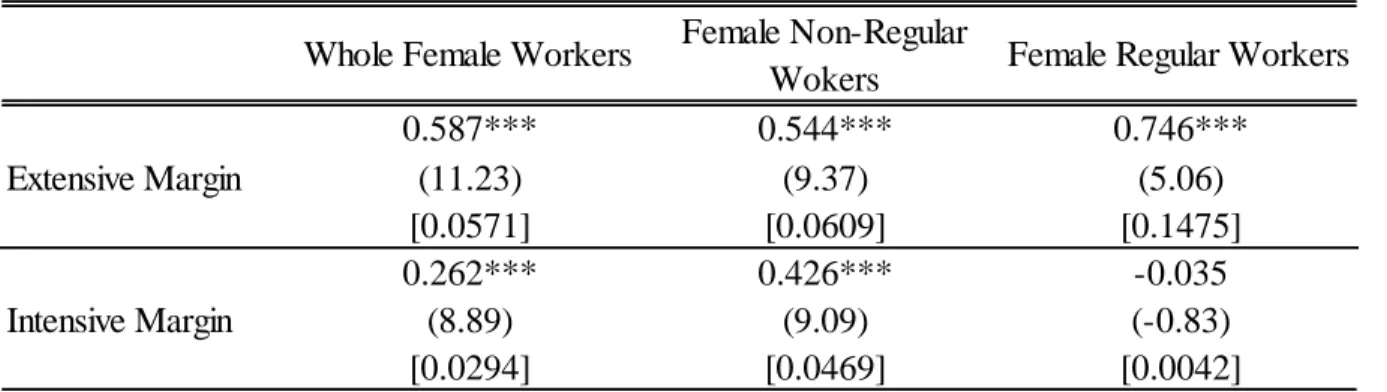
To compare to the female responses, I also calculate both margins of females. Table 4 suggests that female responses of both types of workers are much larger than those of males. This is compatible with findings in Japan and other countries. The interesting feature is that, while the extensive margin of female regular workers is larger than non-regular workers, the intensive margin is as small as male workers. According to Hayashi (2009) who survey labor supply literatures in Japan, for wage elasticity of all females, it is 0.122 on average and extensive margin is 0.107. The results are relatively bigger than the average of Japanese findings, but it is fair to say the values are plausible in other countries’ studies.
Back to the results of male workers, we have to look at this result with a caution, because, even in non-regular work, we can assume there are different working patterns. As
aforementioned, Syokutaku is considered to have quite different working style compared to other non-regular worker. Thus, to distinguish this effect, I will separate data by age groups (under and over 55 years old) to observed more detailed responses.
19
Table 3 Estimated Labor Supply Elasticities aged 18-65 Whole Male Workers Male Non-Regular
Wokers Male Regular Workers
0.0025*** 0.365*** 0.0023*** Extensive Margin (8.79) (9.32) (13.05) [0.0017] [0.0392] [0.0002] 0.009 0.022 0.046 Intensive Margin (1.18) (0.77) (0.56) [0.0070] [0.0288] [0.0083]
a) z-value and t-value are reported in parentheses for extensive and intensive margins respectively. Squared brackets show standard erros.
b) Observations are 4963, 669 and 4626 for extensive margin estimations of each type of workers. For intensive margin estimations, observations are 4631, 337 and 4294.
Table 4 Estimated Labor Supply Elasticities for Women aged 18-65 Whole Female Workers Female Non-Regular
Wokers Female Regular Workers
0.587*** 0.544*** 0.746*** Extensive Margin (11.23) (9.37) (5.06) [0.0571] [0.0609] [0.1475] 0.262*** 0.426*** -0.035 Intensive Margin (8.89) (9.09) (-0.83) [0.0294] [0.0469] [0.0042]
a) z-value and t-value are reported in parentheses for extensive and intensive margins respectively. Squared brackets show standard erros.
b) Observations are 1743, 1494 and 345 for extensive margin estimations of each type of workers. For intensive margin estimations, observations are 2797, 1927 and 870.
20 Estimation results for male workers aged 18-55
Here, I limit my focus on male workers whose age is between 18 and 54 years old eliminating the effect of Shokutaku.
Comparing the previous result, the biggest feature is that the extensive margin of non-regular workers shows much smaller. This is understandable since the prime-age non-regular workers could not get enough money, so that they would be urged to work more, while elder non-regular workers could have received retirement payment, so that their motivation for work would be less than other non-regular workers.
Also, we can see the intensive margin for each worker is decreased (but, all are insignificant).
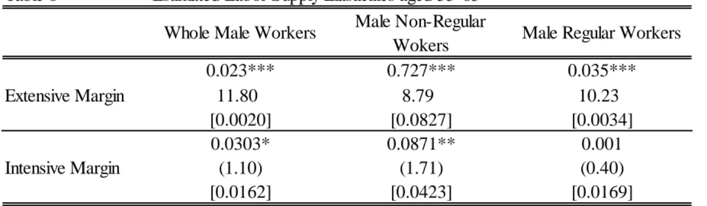
Estimation results for male workers aged 55-65
Table 6 shows elderly worker’s labor supply responses. As we can expect from previous discussions, elderly non-regular workers are sensitive against wage changes in extensive margin. For intensive margin, coefficients become significant for whole and non-regular workers, which
Table 5 Estimated Labor Supply Elasticities aged 18-54 Whole Male Workers Male Non-Regular
Wokers Male Regular Workers
0.0028*** 0.013*** 0.0025*** Extensive Margin (8.44) (4.24) (8.30) [0.0003] [0.0031] [0.0003] 0.003 -0.059 0.003 Intensive Margin (0.27) (1.54) (0.35) [0.0094] [0.0389] [0.0097]
a) z-value and t-value are reported in parentheses for extensive and intensive margins respectively. Squared brackets show standard erros.
b) Observations are 3449, 140 and 3347 for extensive margin estimations of each type of workers. For intensive margin estimations, observations are 3411, 102 and 3309.
21
also ensure flexible working style of Shokutaku. However, still elderly regular worker indicates similar working patterns of that of prime-age males.
6. Conclusion
In this paper, using Japanese micro-panel data (KHPS) from 2004 to 2010, I bring new evidences on Japanese male and female labor supply literatures. In my best knowledge, this is the first comprehensive study for labor supply in Japan.
The obtained results show plausible range of extensive and intensive margins for both workers. While intensive margins of male non-regular and regular workers aged 18 to 65 are quiet small and insignificant, those of females are much bigger as previous literatures suggest. Also, we can see same thing in the extensive margin, that imply females labor decision is much more responsive against wage changes.
The further investigation by separating data to two age groups for males reveals that elderly male non-regular workers are more flexible on their work decision.
Table 6 Estimated Labor Supply Elasticities aged 55-65 Whole Male Workers Male Non-Regular
Wokers Male Regular Workers
0.023*** 0.727*** 0.035*** Extensive Margin 11.80 8.79 10.23 [0.0020] [0.0827] [0.0034] 0.0303* 0.0871** 0.001 Intensive Margin (1.10) (1.71) (0.40) [0.0162] [0.0423] [0.0169]
a) z-value and t-value are reported in parentheses for extensive and intensive margins respectively. Squared brackets show standard erros.
b) Observations are 1514, 529 and 1279 for extensive margin estimations of each type of workers. For intensive margin estimations, observations are 1220, 235 and 985.
22 Summary Statistics
Table7 Summary Statistics for male workers (18-65 years old)
Average S.D Average S.D Average S.D
Before-tax hourly wage 2919.79 2502.81 1756.32 1276.29 3237.53 2499.13
After-tax hourly wage 2128.04 1694.67 1442.17 907.04 2346.89 1679.17
Hours worked per week 44.51 19.40 39.29 15.50 48.13 16.04
Labor Force Participation 0.92 0.27
Non-labor income 73.93 401.06 165.34 436.35 42.37 370.86
Saving 628.94 1034.33 600.23 920.78 578.71 942.19
Age 47.73 9.93 55.25 10.45 46.18 9.10
Tenure 18.28 11.68 16.77 15.21 19.01 10.77
Year of education 13.75 2.26 12.58 2.24 13.93 2.20
Number of Children (< 6 years) 0.28 0.59 0.07 0.30 0.32 0.62
Observations
All men Non-regular worker Regular worker
-
-4964 337 4297
Table8 Summary Statistics for female workers (18-65 years old)
Average S.D Average S.D Average S.D
Before-tax hourly wage 580.80 961.98 741.66 552.00 1928.07 1468.21
After-tax hourly wage 492.05 738.35 681.87 445.89 1514.76 1037.75
Hours worked per week 15.95 19.04 24.83 14.12 41.19 14.65
Labor Force Participation 0.53 0.50
Non-labor income 487.96 474.14 469.30 402.30 363.76 502.66
Saving 709.25 1220.54 469.31 820.03 632.57 946.41
Age 46.93 10.28 46.87 8.67 46.01 9.07
Tenure 5.72 7.40 7.47 5.40 13.95 8.72
Year of education 12.85 1.71 12.73 1.59 13.06 1.76
Number of Children (< 6 years) 0.29 0.60 0.14 0.42 0.19 0.48
Observations 5369 1935 873
-
23 References
1) Asano S. Joint Allocation of Leisure and Consumption Commodities: A Japanese Extended Consumer Demand System 1979-90. The Japanese Economic Review; 48.1; 65-80
2) Bessho S, Hayashi M. Labor Supply Response and Preferences Specification: Estimates for prime-age males in Japan. Journal of Asian Economics 2011; 22; 398-411
3) Bargain O, Orsini K, Peichl A. Comparing Labor Supply Elasticities in Europe and the US: New Results. SOEP papers 2012.
4) Blomquist N. Soren. Labour Supply in a Two-Period Model: The Effect of a Nonlinear Progressive Income Tax. Review of Economic Studies 1985; 52; 515–524.
5) Blundell R, Duncan A, Meghir C. Estimating Labor Supply Responses Using Tax Reforms. Econometrica 1998; 66; 827–861.
6) Dubin J, McFadden D. An Econometric Analysis of Residential Electric Appliance Holdings and Consumption. Econometrica 1984; 52 No. 2, 345-362
7) Genda Y. Shigotono Nakano Aimaina Fuan, Tokyo: Chuokoron Shinsha 2001
8) Heckman JJ. Sample Selection Bias as a Specification Error. Econometrica 1979; 47; 153–161.
9) Heckman JJ, MaCurdy TE. A Life Cycle Model of Female Labour Supply. Revie of Economic Studies 1980. 47 47-74
10) Keane M.P. Labor Supply and Taxes: A Survey. Journal of Economic Literature 2011, 49:4, 961-1075.
24
11) Kimmel J, Kniesner TJ. New Evidence on Labor Supply: Employment versus Hours Elasticities by Sex and Marital Status. Journal of Monetary Economics 1998; 42; 289– 301.
12) Kumar, A.Lifecycle-Consistent Female Labor Supply with Nonlinear Taxes: Evidence from Unobserved Effects Panel Data Models with Censoring, Selection and Endogeneity. Review of Economics of the Household; pp 1-23
13) Kuroda S, Yamamoto I. Estimating Frisch Labor Supply Elasticity in Japan. Journal of the Japanese and International Economies 2008; 22; 566-585
14) Kuroda S, Yamamoto I. Ijitenkan no roudoukyokyuudanseiti no keisoku: wagakuni
yuuhaiguuzyosei no micro-data wo motiita kensyo. Hitotsubashi University Repository
2007. (in Japanese)
15) MaCurdy T, Green D, Paarsch HJ. Assessing Empirical Approaches for Analyzing Taxes and Labor Supply. Journal of Human Resources 1990; 25; 415–490.
16) Ministry of Health, Labour and Welfare in Japan. White Paper on the Labour Economy 2012. in Japanese
17) Semykina A, Wooldridge Jeffrey M. Estimating Panel Data Models in the Presence of Endogeneity and Selection. Journal of Econometrics 2010; 157; 375–380.
18) Yamada T, Yamada T, Kang M. A Study of Time Allocation of Japanese Households. Japan and the World Economy 1999; 11; 41-55
19) Vella F. Estimating Models with Sample Selection Bias: A Survey. The Journal of Human Resources 1998; 33(1); 127-169.
20) Ziliak JP, Kniesner TJ. Estimating Life Cycle Labor Supply Tax Effects. Journal of Political Economy 1999; 107; 326–359.