東北大学機関リポジトリTOUR

(1)

First Data for the Sterile Neutrino Search

using J-PARC MLF Decay at Rest Neutrino

著者

Hino Yota

学位授与機関

Tohoku University

(2)

Detector R&D and Sensitivity Study with the First Data

for the Sterile Neutrino Search using J-PARC MLF

Decay at Rest Neutrino

(J-PARC MLF

からの静止崩壊ニュートリノを用いた

ステライルニュートリノ探索のための

最初のデータを使用した

探索感度の研究と検出器の開発

)

Ph. D. Thesis

Yota Hino

Department of Physics, Tohoku University

(3)

(4)

Abstract

Recently, a variety of neutrino experiments have performed measurement of neu-trino oscillation parameters precisely and constructed strict evidences to the fact that neutrinos have non-zero mass. Diﬀerence between each neutrino ∆m2 is a unique observable related to the information of neutrino mass in neutrino oscillation experiment, and the largest ∆m2reported ever is at most∼ 10−3 eV2. On the other hand, there exists the experimental results: LSND experiment, as a representative, reported muon anti-neutrino to electron anti-neutrino (¯νµ→ ¯νe) oscillation at short

baseline equivalent to ∆m2 > 0.2 eV2 which conflicts the facts reported ever, and it has been left as an anomaly of neutrino oscillation (LSND anomaly).

JSNS2is a neutrino oscillation experiment to search for ¯νµ → ¯νe oscillation

caused by sterile neutrino reported in LSND experiment, which is held in the Mate-rial and Life Science Experimental Facility (MLF) of Japan Proton Accelerator Re-search Complex (J-PARC). The mercury target of MLF prodeuces plenty of ¯νµfrom µ+decay-at-rest (DAR) which well reflects timing structure of low duty factor pro-ton beam so that not only cosmic-ray induced background but also neutrino back-ground from other mother particles, e.g., pion and kaon, using timing imformation. The inverse beta decay (IBD) reaction ¯νe+ p→ e++ n is used to detect ¯νe using

Gadolinium loaded liquid scintillator (Gd-LS): the positron energy proportional to the original neutrino energy, and gamma rays (∼ 8 MeV in total) from thermal neu-tron capture on Gd can also contribute to accidental background reduction in term of energy and shorter timing diﬀerence from the positron timing. These features enable us to perform a direct test to the result of LSND experiment.

The JSNS2_{detector has been constructed recently, and JSNS}2_{experiment just} launched the first data taking on Jun 2020. The data taking period is amount to 10 days equivalent to 1.0 % of the proposed experimental duration, and the data enable us to understand detector response and evaluate the event rate of backgrounds. As a result of the background measurement, we found that cosmic fast neutron gives one of the severe background rate In oreder to recover the situation, we investgated hardware upgrades. Based on the behavior of floor gamma ray, it was found that changing the pattern of the lead brick shield eﬃciently reduces its event rate to 1/6. DIN mixture to the Gd-LS shows good pulse shape discrimnation (PSD) capability to reject fast neutron so that the rejection power to neutron can be enhanced from 100, the current design, to 200.

The In this thesis, studies and works for dector construction are reported. In addition, the background estimation and expected sensitivity of JSNS2experiment based on the real data are shown.

(5)

List of Figures

1.1 Left: a schematic view of the experimental setup of LSND experi-ment. Right: L/E distribution of the observed ¯νe event in LSND

experiment, where L is the baseline, and E is the neutrino energy. The blue area corresponds to the expectation of ¯νe event on the

os-cillation assumption. It describes the data (black point) [3] well. . . 4 1.2 Left: Constraints on short-baseline νµ → νe/¯νµ → ¯νe appearance

oscillations in 3 active + 1 sterile scenario at 99 % C.L.. Right: Com-parison between 99.73 % exclusion limit from disappearance data and the combined allowed region from the appearance data. Their hori-zontal axis shows the eﬀective mixing angle sin22θµe= 4|Ue4|2|Uµ4|2,

and the vertical axis corresponds to ∆m2 [4]. . . 5 1.3 The result of Neutrino-4 experiment [8]. Left: Comparison of the

allowed regions of LSND (1, 2), MiniBooNE (3 - 5) and Neutrino-4 (red contour). 6 and 7 shows KARMEN and OPERA [60] 90 % exclu-sion line, respectively. The parameter sin22θµe∼ 1₄sin22θ14sin22θ24 is determined by the production of sin22θ14 from Neutrino-4 and sin22θ24 from IceCube experiment. Right: Constraints on the pa-rameter space (∆m2, sin22θ14) among various short baseline reactor neutrino experiments. . . 6 2.1 The overview of J-PARC facilities. . . 8 2.2 The MLF building and the location of the JSNS2 experimental setup. 8 2.3 A drawing of the MLF third floor in the bird-eye’s view. The detector

position is pointed as the red box. . . 9 2.4 A cross section of the MLF building in the orthogonal plain to the

beam direction [11]. The red shaded area corresponds to the hot cell where the mercury target is placed. The detector position is pointed as the green box. . . 9 2.5 A cross section of the MLF building in the parallel plain to the beam

direction [12]. . . 10 2.6 A schematic diagram of delayed coincidence IBD detection used JSNS2experiment.

. . . 11 2.7 A schematic view of the JSNS2_detector. _{. . . .} ₁₂ 2.8 A photo of the shield below the JSNS2detector. . . 13 2.9 The detector and LS operation during the experiment throughout a

year [9]. . . 14 2.10 A cut model of an ISO tank with the dimensions labeled [14]. . . . 14 2.11 A schematic drawing of the J-PARC spallation neutron source [10]. 15

(8)

iv LIST OF FIGURES

2.12 A schematic drawing of the mercury target in the J-PARC MLF [10]. 16 2.13 Time distribution of neutrinos from pion, muon and kaon decays.

The origin of the horizontal axis corresponds to beam collision time. Only neutrinos from µDAR survive after 1 µs from the proton beam collision timing [10]. . . 17 2.14 Estimated neutrino flux for all components (left) and components

after 1 µs from proton beam timing (right). As a result of timing selection, the µ+DAR components are selected and main background component is from µ− decays [10]. . . 18 2.15 Feynman diagram of µ+ decay (left) and µ− decay (right). . . 20 2.16 Energy (normalized flux) spectrum of µ+ _{decay (left) and µ}− _decay

(right). . . 20 2.17 Qtail/Qtotal distributions of the IBD events (red) and the cosmic fast

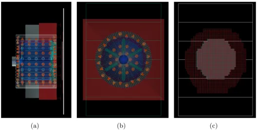
neutron events (blue). . . 23 2.18 The implemented geometry in the JSNS2RAT simulation. (a) size

view, (b) top view, and (c) top view of the shield consist of lead bricks and iron plates . . . 24 2.19 Kinetic energy of positron (red) and neutrino (blue) in IBD

interac-tion. Left: the signal ¯νµ → ¯νe . Right: the background ¯νe from µ−.

. . . 26 2.20 Kinetic energy of generated electron (left) and positron (right) as final

state particles in 12C(νe, e−)12Ng.s. reaction. . . 26

2.21 Cross section of 12C(νe, e−)12Ng.s. reaction. Left: dependence on νeenergy. Right: angle between the νeand the projectile electron [26]. 26

2.22 Reproducibility of the 252Cf generator in the Double Chooz far de-tector [27]. Left: energy distribution for the prompt signal by fission. Right: neutron multiplicity by fission. . . 27 2.23 Left: kinetic energy distribution of generated electron/positron. Right:

2D histogram for generated vertices in the inner detector in zr2 plain. 28 2.24 Generator information of cosmic fast neutron. Top left: kinetic energy

distribution. Top center: cos θ distribution for zenith angle θ. Top right: multiplicity. Bottom left: particle generation point in XY plain. Bottom center: particle generation point in XZ plain. The origin of XYZ coordinate is set to the detector center. . . 29 2.25 A model of concrete walls in the MLF third floor shows spatial

re-lations to the detector in the XZ plane (left) and the YZ plane (right), respectively. We assumes that cosmic ray induced fast neu-tron/gamma ray generated in the concrete volume as a result of an interaction between cosmic muon and matter in the concrete. . . . 30 2.26 Neutron generated position distribution in XY plane (left) and in XZ

plane (right). The origin of XYZ coordinate is set to the detector center. . . 30 2.27 Generator information of cosmic fast neutron. Top left: kinetic energy

distribution. Top right: cos θ distribution for zenith angle θ. Bottom left: particle generation point in XY plain. Bottom right: particle generation point in XZ plain. The origin of XYZ coordinate is set to the detector center. . . 31 2.28 Kinetic energy distribution of floor gamma. . . 32

(9)

3.1 A schematic view of the pulserhead positions and cable routing to the controller box. The blue and violet markers correspond to the visible and UV LEDs, respectively. . . 34 3.2 The emission spectrum of the UV LEDs (left) and the visible LEDs

(right). . . 34 3.3 The timing structure of emitted light pulse of the UV LEDs (left) and

the visible LEDs (right). . . 35 3.4 (a): A drawing of covers for the pulser head made using 3D printer.

In order to avoid cable connector interference the cover separately consists of front and back part. (b): A photo of the LED module installed in the detector. The module and cover are tightly fixed with a bolt and a nut on to the black board, and finally surrounded by reflector sheet. . . 35 3.5 A schematic view of the positions of devices for monitoring. The red

arrows indicates the range of each level sensor or the direction which the web camera looks towards. . . 36 3.6 A block diagram of data acquisition system for sensors and HV [38]. 36 3.7 A screenshot of the grafana page for sensor log. . . 37 3.8 A screenshot of the grafana page for HV log. . . 38 3.9 A photo of the oil test paper before (left) and after oil exposure (right). 38 4.1 (a) History of beam power at MLF in the data taking period.

Aver-aged beam power over a hour is plotted as a function of time in date. Sudden decreases in power were caused by short time beam stop for some reason in the facility side. Note that there was facility mainte-nance beam oﬀ period for 24 hours on June 10. (b) The integrated POT recorded in data. . . 40 4.2 A schematic diagram of DAQ and data flow for the first run. . . 41 4.3 A schematic diagram of timing structure of the kicker trigger. The

red pulse illustrates activity in the detector caused by beam spill to the target, which can be a signal of IBD interaction and so on. . . . 41 4.4 (a) A block diagram of trigger logic for the self trigger. (b) A block

diagram of logic for the online muon veto. . . 42 4.5 A schematic diagram of timing structure of the trigger pulse (top one)

and the associated veto logic pulses illustrated in inverse of the trigger pulse. . . 43 4.6 A history of DAQ eﬃciency in the first run. The total eﬃciency was

94.5%. The eﬃciency loss is caused by setup change and HV crate exchange. . . 44 4.7 An example of waveform with low frequency noise observed during

the dry-run commisionning. The vertical axis indicates pulse heigh in a unit of FADC count. The sharp peak around 700 ns corresponds to a pulse from the LED illumination. . . 45 4.8 An example of hit discrimination using diﬀerential waveform. the top

panel shows a raw waveform recorded at the FADC. Its diﬀerential waveform is displayed in the bottom panel. The red line in the bottom panel exhibits threshold level to discriminate single p.e. hit. . . 45

(10)

vi LIST OF FIGURES

4.9 Left: a correlation between pulse height of diﬀerential waveform (hor-izontal axis) and that of raw waveform (vertical axis). The red dashed line corresponds to the threshold level for the single p.e. hit discrimi-nation. Right: pulse height distributions of all events (black markers) and events with hit (red markers). The blue line shows a fit result with an exponential and gaussian function as a model for single p.e.. 46 4.10 Left: single p.e. detection eﬃciency of the hit discrimination

con-dition for each ID PMT. Right: the distribution of the single p.e. detection eﬃciency. It indicates that the condition can ensure at least 60 % eﬃciency for single p.e. detection over the PMTs. . . 46 4.11 Top: the total number of p.e. distributions of all generate events (red)

and the events with more than 20 hit. Note that they are obtained from the MC simulation of neutron capture events. The peaks at

∼ 250 and ∼ 900 p.e. correspond to nH and nGd peak, respectively.

Bottom: the eﬃciency of the event definition condition (the number of hit > 20) as a function of the total number of p.e.. The eﬃciency reaches to 99 % at 100 p.e. equivalent to 1 MeV. . . 48 4.12 An example of number of hit waveform. The dashed rectangles

col-ored green, blue and orange indicate the defined event windows. The red solid box shows beam on-bunch timing region. . . 49 4.13 Top: the total number of p.e. distributions of all events (red) and the

events with more than 80 mV A.S.PH (blue). Bottom: the trigger eﬃciencies of all events (black line), events in the top half volume (red) and events in the bottom half volume (blue) as a function of the total number of p.e.. The eﬃciencies are consistent with 100 % above 450 p.e. equivalent to 4 MeV. . . 50 4.14 (a) The definition of variables computed from a waveform. (b) an

example of CFD waveform. The red point indicates zero crossing point used as timing. . . 51 4.15 An example waveform of kicker (blue) and CT (red) pulses. The

vertical axis corresponds to pulse height in a unit of FADC count, and the horizontal axis shows time in a unit of nano second. The CT pulse has 2 bunch structure reflecting the proton beam spill. . . 51 4.16 Left: Charge distribution of PMT No.4 in the inner detector as a

result of gain calibration run using LED 12. Right: Charge distribu-tions PMT No.103 in the veto layer. The blue marker shows data, and green line represents fitting result with single gaussian. . . 53 4.17 Gain distribution for all PMTs. The blue shaded one shows gain

distribution of the inner PMTs, and the green one is for veto PMTs. 54 4.18 Correlation between NPE ratio of LG to HG and NPE in high gain

channel assuming that the typical gain of FEE is 0.7 and 16 for low gain and high gain, respectively. The dashed green line exhibits the selection region for correction factor computation. . . 55 4.19 A schematic diagram of timing calibration using the nano-pulser LED

(11)

4.20 (a) A histogram of timing difference between signal on PMT 7 and external trigger pulse from LED 4. (b) Relative timing difference for all PMTs. Trigger timing difference unique to each LED are corrected using timing of the overlapped PMTs. The origin in the vertical axis is arbitrary; however, the relative values among PMTs are calibrated. The colors of marker classify cable length of PMT. . . 57 4.21 Event selection criterion displayed by blue dashed box for the data

(a) and the MC (b), respectively. . . 57 4.22 A map of the PMT groups. . . 58 4.23 The observed NPE response of each PMT group when the252Cf source

deployed at the center (z = 0 cm). Both response of the data (black dots) and the MC (red dashed line) are overlaid to compare them. . 58 4.24 The observed NPE response of each PMT group when the252Cf source

deployed at z = 50 cm (left) and -50 cm (right). Both response of the data (black dots) and the MC (red dashed line) are overlaid to compare them. . . 59 4.25 The observed NPE response of each PMT group when the252Cf source

deployed at z = +75 cm (left) and -75 cm (right). Both response of the data (black dots) and the MC (red dashed line) are overlaid to compare them. . . 59 4.26 The observed NPE response of each PMT group when the252Cf source

deployed at z = +100 cm (left) and -100 cm (right). Both response of the data (black dots) and the MC (red dashed line) are overlaid to compare them. . . 60 4.27 An example of the response map of the group top 0. The vertical and

horizontal axes correspond to a distance between a vertex and PMT

r and cos θ of a zenith angle to the vertex θ. The z axis exhibited as

color graduation represents expected number of p.e. per MeV at each vertex. . . 61 4.28 A schematics of the coordinate in the response map. . . 61 4.29 The measured PMT response representing a saturation eﬀect in 10

inch PMT R7081 at the gain of the inner PMT [46]. The red points are the measured data, the black line indicates the fitting result based on the model function ginve by Eq. (4.12), respectively. The uncertainty of the fitting is displayed as the green area. . . 62 4.30 Left: selection criteria for cosmic muon tagging. Events in the outside

of the red dashed box are defined as activities caused by cosmic muon. Right: Energy distribution in common logarithm scale before (black) and after muon veto (red) in the horizontal axis. . . 63 4.31 Correlation between pulse height of the veto top analog sum signal

(vertical) and total charge in the veto layer QVeto_total (horizontal). The former is used for online muon veto by applying 75 mV threshold equivalent to 200 p.e.. . . 64

(12)

viii LIST OF FIGURES

4.32 Delayed coincidence for the data with the 252Cf source positioned at z = 0 cm along the z axis. Top left: prompt visible energy. Top right: delayed visible energy. Middle left: ∆tp−d. Middle right: ∆V T Xp−d. Bottom left: multiplicity of delayed signal. Bottom right: total charge in the veto layer. Each distribution of variable is applied all selections except for the selection to itself. The red boxes show the selection cri-terion to each variable. The green marker corresponds to correlated event candidates, and the blue one shows the estimated accidental co-incidence events. The accidental subtracted distribution is displayed as the black marker in the plots. . . 66 4.33 A schematic of delayed coincidence for correlated events. Accidental

coincidence is estimated using oﬀ timing window. . . 67 4.34 Time constant τ as a result of the fitting to the ∆tp−d distribution

with an exponetial function at each source position. They are in agreement within 2 % each other. . . 67 4.35 Left: the delayed energy spectrum with the nGd and nH peak fittings

in case the source is at Z = 0 cm. Right: the energy resolution at each position as a function of the visible energy. . . 68 4.36 Delayed visible energy (left) and ∆t distribution (right) at z = 0 cm.

The black marker shows the data points after accidental subtraction. The blue shaded histogram is the MC simulation output. . . 69 4.37 Delayed visible energy (left) and ∆t distribution (right) at z = +50,

+75, +100 cm from the top. The black marker shows the data, and the blue shaded area corresponds to the MC simulation output, re-spectively. . . 70 4.38 Delayed visible energy (left) and ∆t distribution (right) at z = -50,

-75, -100 cm from the top. The black marker shows the data, and the blue shaded area corresponds to the MC simulation output, respec-tively. . . 71 4.39 The selection eﬃciency of delayed visible energy (left) and that of ∆t

selection (right) at each source position. The eﬃciencies estimated based on the data (black) and the MC simulation (blue) are displayed simultaneously. . . 72 4.40 Comparisons of the reconstructed vertex between data and MC at z

= 0 cm. Top: x, middle: y, bottom: z of the reconstructed vertex, respectively. . . 72 4.41 Diﬀerence of reconstructed vertex between data and MC about z at

various source positions. They agreed with each other within ± cm diﬀerence over the range. . . 73 4.42 Delayed coincidence for Michel electron selection. Top left: prompt

visible energy. Top right: delayed visible energy. Middle left: ∆tp−d. Middle right: ∆V T Xp−d. Bottom left: multiplicity of delayed signal. Bottom right: total charge in the veto layer. Each distribution of variable is applied all selections except for the selection to itself. The red boxes show the selection criterion to each variable. The green marker corresponds to correlated event candidates, and the blue one shows the estimated accidental coincidence events. The accidental subtracted distribution is displayed as the black marker in the plots. 75

(13)

4.43 Fitting result to ∆tp−d distribution with an exponential function ex-hibited as the blue line. The black marker shows the accidental-subtracted histogram identical with the middle left plot in Fig. 4.42.

. . . 76 4.44 Left: the fitting result (blue line) to the Michel electron spectrum

obtained from the data (black markers). Right: ∆χ2 _{curve of the} fitting. The estimated constant term is 4.61+0.20_−0.18 %, which can be interpreted as an averaged value over the target volume. . . 77 4.45 Comparative plots of Michel electron events between data and MC

simulation. Top left: the visible energy spectrum. Top right: Z distribution. Bottom left: ρ =√x2_{+ y}2 _{distribution. Bottom right:} R =√x2_{+ y}2_{+ z}2 _{distribution. The black marker shows spectrum} of the accidental-subtracted data, and the blue shaded area is that of the MC simulation. . . 77 4.46 Delayed coincidence for cosmic fast neutron selection to the data

ob-tained using the self trigger without the online veto. Top left: prompt visible energy. Top right: delayed visible energy. Middle left: ∆tp−d. Middle right: ∆V T Xp−d. Bottom left: multiplicity of delayed signal. Bottom right: total charge in the veto layer. Each distribution of variable is applied all selections except for the selection to itself. The red boxes show the selection criterion to each variable. The green marker corresponds to correlated event candidates, and the blue one shows the estimated accidental coincidence events. The accidental subtracted distribution is displayed as the black marker in the plots. 79 4.47 Delayed coincidence for cosmic fast neutron selection to the data

ob-tained using the self trigger with the online veto. Top left: prompt visible energy. Top right: delayed visible energy. Middle left: ∆tp−d. Middle right: ∆V T Xp−d. Bottom left: multiplicity of delayed signal. Bottom right: total charge in the veto layer. Each distribution of variable is applied all selections except for the selection to itself. The red boxes show the selection criterion to each variable. The green marker corresponds to correlated event candidates, and the blue one shows the estimated accidental coincidence events. The accidental subtracted distribution is displayed as the black marker in the plots. 80 4.48 Distributions of prompt visible energy (top left), delayed visible

en-ergy (top right), ∆t (bottom left), and ∆V T X (bottom right). The blue shaded area shows MC output of each variable overlaid with the data (black marker) in order to compare them. . . 81 4.49 The event vertex distribution in the detector. The histograms of z,

ρ =√x2_{+ y}2 _{and R =}√_x2_{+ y}2_{+ z}2 _{are placed in the order of the} top to the bottom. The plots in the left hand size corresponds to the histogram of the prompt signal, and the plots in the right hand side shows that of the delayed signals, respectively. The blue shaded area shows MC output of each variable overlaid with the data (black marker) in order to compare them. . . 82

(14)

x LIST OF FIGURES

4.50 Left: the single rate energy spectrum in the beam oﬀ period (black marker) with its components classified by color. Right: the residual energy spectrum after subtraction (green marker) corresponding to the green shaded area in the left plot. The overlaid spectrum (blue shaded area) shows the MC simulation of cosmic gamma, and consis-tently agree with the residual spectrum from the data above 5 MeV.

. . . 84 4.51 Left: Correation between visible energy and event timing of the prompt

signal. Right: Correation between visible energy and event timing of the delayed signal. The origin of the horizontal axes in each plot are set to the beam timing. The red dashed boxes show the selection criteria to the prompt andthe delaeyd signal, respectively. . . 85 4.52 Delayed coincidence for nGd events correlated to on-bunch neutron in

run 1416. Top left: prompt visible energy. Top right: delayed visible energy. Middle left: ∆tp−d. Middle right: ∆V T Xp−d. Bottom left: multiplicity of delayed signal. Bottom right: total charge in the veto layer. Each distribution of variable is applied all selections except for the selection to itself. The red boxes show the selection criterion to each variable. The green marker corresponds to correlated event candidates, and the blue one shows the estimated accidental coinci-dence events. The accidental subtracted distribution is displayed as the black marker in the plots. . . 86 4.53 The prompt vertex (left) and the delayed vertex distribution (right)

in the XY plane. The biased vertex distributions in y > 0 cm region reflects the incoming direction of beam on-bunch fast neutron. The marcury target exists in the +y direction in the ditector coordinate. 87 4.54 The nGd event subtraction from single rate spectrum in run 1416 for

example. Left: all range. Right: zoomed into the red arrow region in the left plot. . . 87 4.55 The nGd event subtracted spectrum (black marker) for all runs listed

in table 4.6. The spectrum shape is described by floor gamma (blue shaded area), cosmic gamma (red shaded area) and Michel electron (green shaded area) in the range of 4 to 100 MeV. . . 88 4.56 ∆V T XOB−d distribution in the condition 7 < EvisID < 12 MeV when

on-bunch event exists. The beam unrelated events, e.g., IBD and cos-mic fast neutron, belongs to the accidental distribution (blue mark-ers). The black marker distribution shows nGd events correlated with beam on-bunch neutron. . . 91 4.57 A schematic of algorithm for accidental coincidence estimation. . . 91 4.58 Delayed coincidence for the IBD event selection. Top left: prompt

visible energy. Top right: delayed visible energy. Middle left: ∆tp−d. Middle right: ∆V T Xp−d. Bottom left: ∆V T XOB−d. Each distri-bution of variable is applied all selections except for the selection to itself. The red boxes show the selection criterion to each variable. The green marker corresponds to correlated event candidates, and the blue one shows the estimated accidental coincidence events. The accidental subtracted distribution is displayed as the black marker in the plots. . . 92

(15)

4.59 Correlation between ∆tbeam−p (vertical axis) and ∆tp−d (horizontal axis). The FADC window size (25 µs ) naturally limits timing infor-mation used in the selection. . . 93 5.1 The measured timing profile of the proton beam to the mercury

tar-get [55]. . . 98 5.2 Left: The timing profile of signal as a function of signal timing with

respect to beam timing. Right: The estimated signal eﬃciency as a function of end point of the selection criterion. The red line indicates the eﬃciency value in case of 1.5 < ∆tbeam−p < 10 µs . . . . 98 5.3 Correlations between ∆tbeam−p (vertical axis) and ∆tp−d (horizontal

axis) of the singal (top), the accidental backgrounds (middle), and cosmic fast neutron events (bottom). . . 100 5.4 Top: distributions of log-likelihood value, middle: selection eﬃciency

as a function of selection value of log-likelihood for the signal (red), the accidental events (green) and cosmic fast neutron (blue). Bottom: the enhance curves of signal to accidental (green) and signal to fast neutron (blue). . . 101 5.5 Top: The delayed energy distribution of the IBD simulation (black)

and the accidental events during beam operation (green). Middle: selection eﬃciency as a function of the endpoint of the delayed energy selection of signal (black) and background (green). Bottom: The enhance curve of signal to accidental background eﬃciency. . . 103 5.6 ∆tp−d distribution of the data with 252Cf at the Z = 0 cm (black

marker) and the signal MC output. . . 104 5.7 Prompt visible energy spectra of the signal (blue shaded arae) and

the background IBD events (orange line). The red dashed box corre-sponds to the selection criterion. The selection eﬃciencies are 95.5 % for the signal and 93.4 % for the background IBD, respectively. Note that the signal spectrum shows the 100 % oscillation case. . . 105 5.8 Top: Distributions of ∆V T XOB−d for the correlated delayed event

with on-bunch activity (black) and the events accidentally coincided with on-bunch activity (blue). Note that the signal IBD will be acci-dental in this case. Middle: eﬃciency curves as a function of cut line of the selection to the signal (blue) and the on-bunch correlated event (black). Bottom: enhance curve of signal to on-bunch correlated de-layed event. . . 106 5.9 Top: ∆V T Xp−d distribution of the fast neutron sample (red marker)

and the accidental sample (green) in the data, respectively. The blue dashed line shows that of the IBD from the signal MC simulation. Middle: eﬃciency curves as a function of cut line of the selection in the same color classification. Bottom: enhance curves: signal to fast neutron (red), signal to accidental (blue) and fast neutron to accidental (green). Spike on the curves is due to poor statistics below 80 cm. . . 108

(16)

xii LIST OF FIGURES

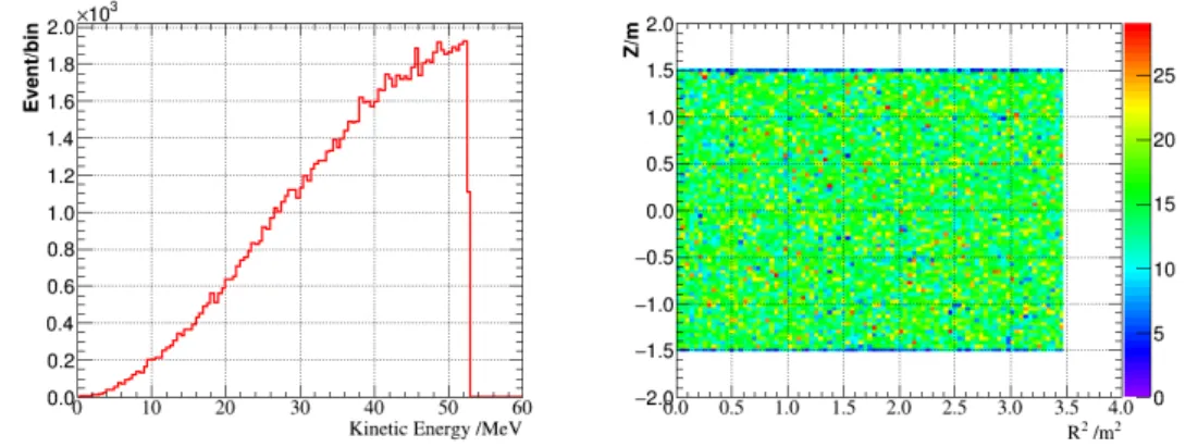
5.10 MC simulation result in the current JSNS2shield configuration. Left: True deposited energy in the detector. Right: Event vertex distribu-tion in the detector. The horizontal axis shows r2 of the vertex, and the vertical axis corresponds to z of the vertex. The gray rectangles illustrate the lead shield coverage. . . 111 5.11 MC simulation result in the upgraded shield configuration. Left: True

deposited energy in the detector. Right: Event vertex distribution in the detector. The horizontal axis shows r2 of the vertex, and the vertical axis corresponds to z of the vertex. The gray rectangles illustrate the lead shield coverage. . . 111 5.12 (a) A photo of the setup for PSD capability measurement. 100 mL

of each DIN mixed Gd-LS sample contained in the 2 inch vial was exposed to 252Cf source, and 10 inch PMT (R7081) observed scin-tillation light from the sample. (b) Definition of variables especially

Qtail. The integration range is from 30 ns to 200 ns after the peak. 112 5.13 The results of PSD capability measurement for each sample. Top

panel shows a correlation of Qtail/Qtotal(vertical axis) and Qtotal (hor-izontal axis). The bottom panel displays Qtail/Qtotal distribution in the selection region (600 - 1200 p.e.) shown in the top panel. . . 113 5.14 The estimated PSD capability of the DIN mixed Gd-LS in the JSNS2detector.

Left: Qtail/Qtotalversus Qtotal in the unit of the nuber of p.e.. Right:

Qtail/Qtotal distribution in the prompt signal region. The balck line

shows the criterion at neutron rejection power 200. . . 113 5.15 The measured transmittance spectrum. The top panel shows raw

transmittance spectra of the DIN mixed sample measured in the first day (black) and 23 day later (red). The bottom panel displays the ratio spectrum of the red one to the black one as a function of wave-length. The drop below 410 nm is because of divergence of the ratio.

. . . 114 5.16 The delayed coincidence of νe+12C→ e−+12Ng.s.. Top left: prompt

energy spectrum. Top right: delayed energy spectrum. Bottom left: ∆V T Xp−d distribution. Bottom right: ∆V T Xp−d distribution. The red dashed boxes on each plot show selection criteria to each variable. 116 5.17 Top: Expected energy spectrum of prompt signal in the current

con-figuration. Bottom: that of the upgraded configuration in the condi-tion of 1 MW× 3 years × 1 detector. The oscillated signal in case of

(∆m2, sin22θ) = (2.5 eV2, 3.0×10−3) (brown shaded area), the IBD

of ¯νe from µ− (red), νe+12C→ e−+12Ng.s.(blue), cosmic fast neu-tron (green) and total accidental background (orange) are displayed together. The spectrum shown in the black points corresponds to the summation of all spectra. . . 120

(17)

5.18 Top: Expected energy spectrum of prompt signal in the current con-figuration. Bottom: that of the upgraded configuration in the condi-tion of 1 MW× 3 years × 1 detector. The oscillated signal in case of

(∆m2, sin22θ) = (1.2 eV2, 3.0×10−3) (brown shaded area), the IBD

of ¯νe from µ− (red), νe+12C→ e−+12Ng.s.(blue), cosmic fast neu-tron (green) and total accidental background (orange) are displayed together. The spectrum shown in the black points corresponds to the summation of all spectra. . . 121 5.19 Sensitivity of JSNS2_{experiment based on the real data. 90% C.L.}

exclusion lines of the expectation in reference [9] (black), the up-graded configuration (red) and the current configuration (green) are displayed. The star points at the parameters of LSND best-fit. The exclusion line of the OPERA experiment is also shown [60]. . . 122 5.20 90% C.L. exclusion to 3 + 1 sterile oscillation from JSNS2experiment

in case of 3 years (blue), 6 years (green) and 8 years experimental duration (red) after the upgrade. It is turned out that 6 years experi-mental duration improves the sensitivity within 19 % loss with respect to the designed performance on sensitivity in reference [9] (black). . 122 5.21 A comparison between the global fit result (red region) and 90% C.L.

(orange), 99 % C.L. sensitivities of JSNS2_{experiment in case of 3} years experimental duration after the upgrade. It is shown that the sensitivity is insuﬃcient to cover the global fit favored region even it can reach to the KARMEN exclusion limit [5]. . . 123 5.22 A comparison between the global fit result (red region) and 90% C.L.

(orange), 99 % C.L. sensitivities of JSNS2experiment in case of 6 years experimental duration after the upgrade. Extending the experimental duration from 3 to 6 years gives a slight improvement. . . 123 6.1 A schematic view of the detectors in NA61/SHINE experiment [62]. 126 6.2 The planned detector location for the far detector with 48 m baseline. 127 6.3 A schematic design of the far detector. The basic design is identical

with the near detector. . . 128 6.4 A model of concrete walls around the far detector cite shows spatial

relations to the far detector in the XZ plane (left) and the YZ plane (right), respectively. We assumes that cosmic ray induced fast neu-tron/gamma ray generated in the concrete volume as a result of an interaction between cosmic muon and matter in the concrete. . . . 129 6.5 The MC simulation results of the cosmic fast neutron. Prompt energy

spectra (top left), delayed energy spectra (top right), ∆t distributions (bottom left), ∆V T X distributions (bottom right) of the near detec-tor (black line) and the far detecdetec-tor (blue line), respectively. The red dashed boxes show the selection criteria for each variables. . . 130 6.6 The MC simulation result of the cosmic gamma ray. The energy

spectra in the prompt energy range (left) and in the delayed energy (right) of the near detector (black line) and the far detector (blue line) are shown, respectively. The red dashed boxes show the selection criteria for each variables. . . 131

(18)

xiv LIST OF FIGURES

6.7 Top: Expected prompt energy spectrum of the near detctor for 8 years. Rihgt: that of the far detector for 5 years. The oscillated sig-nal in case of (∆m2, sin22θ) = (2.5 eV2, 3.0× 10−3) (brown shaded area), the IBD of ¯νe from µ− (red), νe+12C → e−+12Ng.s. (blue), cosmic fast neutron (green) and total accidental background (orange) are displayed together. The spectrum shown in the black points cor-responds to the summation of all spectra. . . 132 6.8 Top: Expected prompt energy spectrum of the near detctor for 8

years. Rihgt: that of the far detector for 5 years. The oscillated sig-nal in case of (∆m2, sin22θ) = (1.2 eV2, 3.0× 10−3) (brown shaded area), the IBD of ¯νe from µ− (red), νe+12C → e−+12Ng.s. (blue), cosmic fast neutron (green) and total accidental background (orange) are displayed together. The spectrum shown in the black points cor-responds to the summation of all spectra. . . 133 6.9 A comparison between the global fit result (red region) and 90% C.L.

sensitivities of the JSNS2-II configuration in case the uncertainty on ¯

νefrom µ− flux are 50 % (green dashed line), 20 % (light blue dashed

line) and 10 % (magenta line) are shown. . . 134 6.10 A comparison between the global fit result (red region) and 3σ C.L.

sensitivities of the JSNS2-II configuration in case the uncertainty on ¯

νefrom µ− flux are 50 % (green dashed line), 20 % (light blue dashed

(19)

List of Tables

2.1 Classification of Beam Neutrinos. . . 18

2.2 An estimate of µDAR neutrino production by 3 GeV protons using FLUKA hadron simulation package [10]. . . 18

2.3 An estimate of µDAR neutrino production by 3 GeV protons using QGSP-BERT hadron simulation package [10]. . . 19

2.4 IBD selection conditions and their eﬃciencies in the JSNS2experiment [9]. . . . 21

2.5 The optical parameters used in the JSNS2RAT simulator. . . 24

3.1 List of devices for monitoring. . . 37

4.1 Trigger menu for the first run. . . 43

4.2 Table of LED intensity for gain calibration. . . 53

4.3 Table of LED intensity for gain calibration. . . 54

4.4 Table of LED intensity for relative timing calibration. . . 56

4.5 The estimated constant term from the252Cf data. . . 68

4.6 Run list for floor gamma estimation. . . 84

4.7 The results of floor gamma estimation for each run. . . 89

4.8 Run list for event rate estimation. . . 89

4.9 A summary of background measurement for each component. . . . 94

5.1 Component classification in lifetime. . . 99

5.2 Eﬃciencies of lifetime cut. . . 99

5.3 Eﬃciencies of delayed energy selection. . . 102

5.4 Eﬃciencies of ∆V T XOB−d selection. . . 105

5.5 Eﬃciencies of ∆V T Xp−d cut. . . 107

5.6 A summary of signal eﬃciency estimation. . . 109

5.7 Summary of the expected number of events for 5000 hours × 3 years. 118 6.1 Summary of the expected number of events for 5000 hours× 8 years for the near detector and 5 years for the far detector, respectively. . 129

(20)

Chapter 1

Introduction

1.1 Neutrino Oscillation

While neutrino mass is zero in the standard model of elementary particles. It has been turned out that neutrinos have finite but small mass from observations of neutrino oscillation. The transition among flavor eigenstates occurs if they con-sist of superposition of mass eigenstates with non-zero mass. This phenomenon in neutrinos is called neutrino oscillation. The mixing of mass eigenstate and three flavor neutrinos in thestandard model (νe, νµ, ντ) is described by

Pontecorvo-Maki-Nakagawa-Sakata (PMNS) Matrix [1], U , as follows:  _|ν|ν_µe⟩_⟩ |ντ⟩   = U∗  |ν_|ν1₂⟩_⟩ |ν3⟩   =  U ∗ e1 Ue2∗ Ue3∗ U_µ1∗ U_µ2∗ U_µ3∗ U_{τ 1}∗ U_{τ 2}∗ U_{τ 3}∗    |ν_|ν1₂⟩_⟩ |ν3⟩   , (1.1)

where|να⟩ (α = e, µ, τ) and |νi⟩ (i = 1, 2, 3) are flavor and mass eigenstates,

respec-tively. U_αi∗ is the complex conjugate of the matrix element. The PMNS matrix is parametrized by U =  10 c023 s023 0 −s23 c23     c13 0 s13e −iδ 0 1 0 −s13eiδ 0 c13    _−sc12₁₂ sc1212 00 0 0 1   =   c12c13 s12c13 s13e −iδ −s12c23− c12s23s13eiδ c12c23− s12s23s13eiδ s23c13 s12s23− c12c23s13eiδ −c12s23− s12c23s13eiδ c23c13   , (1.2)

where sij = sin θij and cij = cos θij. θij(i, j = 1, 2, 3) stand for mixing angles

between νi and νj. There is a phase factor δ expressing the CP violation in lepton

sector. If neutrinos are Majorana particles, two additional phase factors, Majorana phase, appear in the matrix. However, they have no contribution to the oscillation probability described below because it is proportional to UαjUβj∗ Uαk∗ Uβk.

Non-zero mixing causes neutrino flavor transition as a function of time. The time evolution of neutrino with definite mass and energy in vacuum is written by Schr¨odinger equation as

i∂

∂t|νi(t)⟩ = H |νi(t)⟩ = Ei|νi(t)⟩ , (1.3)

(21)

where Ei is the energy of the neutrino νi and H is the Hamiltonian operator in

vacuum. Its solution is given by

|νi(t)⟩ = |νi(t = 0)⟩ e−iEit. (1.4)

Therefore, the propagation of a flavor eigenstate α is expressed using the eigenstate of the other flavor β as

|να(t)⟩ = 3 ∑ i=1 U_αi∗ |νi(t = 0)⟩ e−iEit =∑ β 3 ∑ i=1

U_αi∗Uβi|νβ(t = 0)⟩ e−iEit.

(1.5)

And then, the probability of the flavor transition, να to νβ, is calculated as P (να→ νβ) =| ⟨νβ| να(t)⟩ |2 = 3 ∑ i=1 3 ∑ j=1

UαiUβi∗Uαj∗ Uβje−i(Ei−Ej)t.

(1.6)

Because it is possible to assume that the neutrino mass is negligibly small compared to the momentum of neutrino in ordinary experimental conditions, the neutrino energy in the mass eigenstate i can be approximated by

Ei = √ |p|2_{+ m} i2 ∼ |p| + mi2 |p| ∼ E + 1 2Eν mi2, (1.7)

where Eν is the neutrino energy. Therefore, Eq. (1.6) can be rewritten using

∆m2/2Eν ≡ (mi2− mj2)/2Eν ∼ Ei− Ej and flight length of the neutrino L∼ t (in

the unit of c = 1) as P (να → νβ) = 3 ∑ i=1 3 ∑ j=1

UαiUβi∗Uαj∗ Uβje−i ∆mij2L

4Eν

= δαβ− 4

∑

i<j

Re(UαiUβi∗Uαj∗ Uβj) sin2

( ∆mij2L 4Eν ) + 2∑ i<j

Im(UαiUβi∗Uαj∗ Uβj) sin

( ∆mij2L 2Eν ) , (1.8)

where δαβ is the Kronecker delta. The phase of oscillation Φij can be expressed in

the diﬀerent unit system for convenience by explicitly considering c and ℏ as Φij = ∆mij2c4L 4ℏcEν = 1.27×∆mij 2[_eV2]_{× L [m]} Eν[MeV] . (1.9)

1.1.1 Sterile Neutrino in 3 + 1 model

The current knowledge about neutrino mass from the neutrino oscillation observation is listed below [2]:

∆m212 = (7.42+0.21_−0.20)× 10−5eV2,

∆m312 = (2.517+0.026_−0.028)× 10−3eV2 (Normal Hierarchy), ∆m322 = (2.498+0.028_−0.028)× 10−3eV2 (Inverted Hierarchy).

(22)

1.2. SITUATION FOR STERILE NEUTRINO SEARCH 3 In contrast, the observations of ¯νµ → ¯νe oscillation in LSND (Liquid Scintillator

Neutrino Detector) experiment [3] suggests an existence of oscillation corresponding to ∆m2 ∼ 1 eV2 which conflicts with the measured ∆m2of three neutrinos in the standard model. This is called LSND anomaly. According to the measurement of the probability of e+ + e− → Z0 → ν + ¯ν reaction, the number of generation of weakly interacting neutrino is limited to 3. Therefore, it is necessary to introduce a non-weakly interacting neutral lepton mixing with the three active neutrinos via neutrino oscillation in order to describe the LSND oscillation. It is called sterile neutrino. Assuming the number of sterile neutrino is 1, i.e., 3 + 1 model, the PMNS matrix can be extended as

    νe νµ ντ νs     = U′     ν1 ν2 ν3 ν4     =     Ue1 Ue2 Ue3 Ue4 Uµ1 Uµ2 Uµ3 Uµ4 Uτ 1 Uτ 2 Uτ 3 Uτ 4 Us1 Us2 Us3 Us4     , (1.11)

where νs shows a neutrino in the sterile flavor, and ν4 is an additional mass eigen-state. The probability of oscillation ¯νµ → ¯νe reported by LSND experiment is

written as P (νµ→ νe) =− 4 ∑ j>k Re(UejUµj∗ Uek∗ Uµk) sin2∆jk − 2∑ j>k Im(UejUµj∗ Uek∗Uµk) sin 2∆jk, (1.12) where ∆jk ≡ (mj2− mk2)L 4E . (1.13)

Assuming m4 ≫ m1,2,3 and Us4 ∼ 1 ≫ Uf 4(f = e, µ, τ ), Eq. (1.12) can be

approxi-mated by P (νµ→ νe)∼ 4|Ue4|2|Uµ4|2sin ( ∆m2L 4E ) , = sin22θ sin ( 1.27∆m2[eV2]× L [m] E [MeV] ) , (1.14)

where ∆m2 ∼ m4. Note that the production of transition amplitudes are replaced with a mixing parameter as sin22θ, and the unit of the phase is changed in the same way as Eq. (1.9).

1.2 Situation for Sterile Neutrino Search

As mentioned above, LSND reported the positive result on ¯νµ → ¯νe appearance

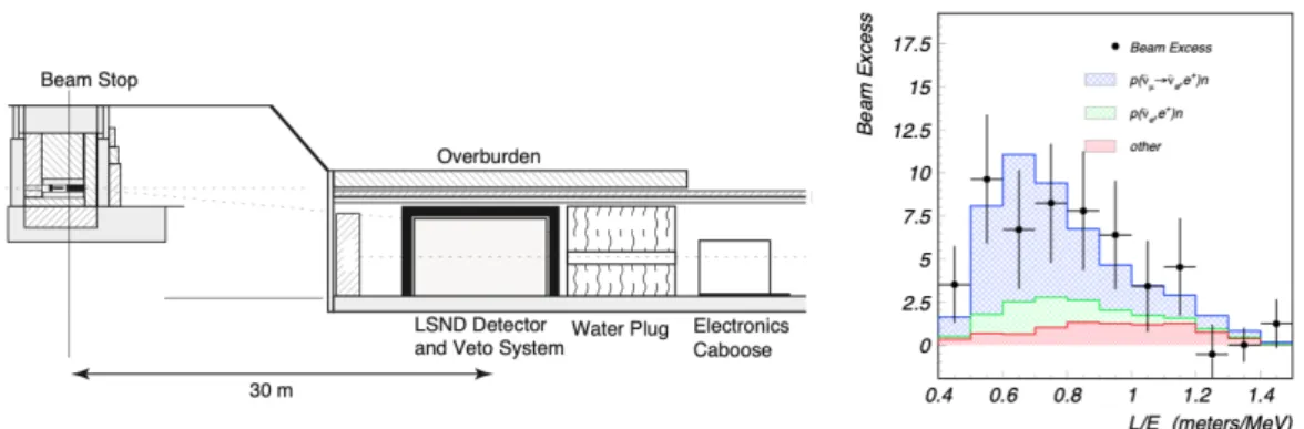
oscillation. They utilezed ¯νµbeam produced in µ decay at rest: π−→ µ−+¯νµ; µ−→ e−+ ¯νe+ νµ using 800 MeV proton beam in LAMPF (Los Alamos Meson Physics

Facility). The experimental setup, shown as the left drawing in figure 1.1, consists of a 176 tons liquid scintillator detector placed at 30 m away from the beam target. The right plot in figure 1.1 shows L/E distribution of the observed ¯νeevents detected

(23)

Figure 1.1: Left: a schematic view of the experimental setup of LSND experiment. Right: L/E distribution of the observed ¯νe event in LSND experiment, where L

is the baseline, and E is the neutrino energy. The blue area corresponds to the expectation of ¯νe event on the oscillation assumption. It describes the data (black

point) [3] well.

against backgrounds (blue shaded area), which corresponds to the allowed oscillation parameters ∆m2> 3× 10−2 eV2, sin22θ > 10−3 [3].

There have been experiments searching for νµ → νe (¯νµ → ¯νe ) oscillation

re-ported in LSND. Figure 1.2 (a) shows the oscillation parameter space of νµ → νe

and ¯νµ→ ¯νe oscillation from results of various experiments at 99 % confidence level

(C.L.) [4]. Even though the negative result from KARMEN [5] (blue dashed line) and OPERA [6] (purple line) gives strong constraints on the positive result from LSND and MiniBooNE [7], the allowed parameter space (red area) survives and indicates an oscillation caused by sterile neutrino.

In addition to the appearance observation, νe (¯νe ) and νµ (¯νµ ) disappearance

data can also give constraints on the survived region from the appearance global fit. Figure 1.2 (b) displays 99.73 % C.L. exclusion line (blue) to the parameter space around the survived region from the appearance data result [4]. Although there is an uncertainty from reactor neutrino flux in ¯νe disappearance experiments,

it gives strong tension between the appearance and the disappearance channel and excludes the favored oscillation by LSND + MiniBooNE at the 4.7 σ level. On the other hand, recently Neutrino-4 experiment, short baseline ¯νe disappearance

measurement using reactor neutrino, reported a positive result at 1 σ level around the LSND+MiniBooNE indicated parameters (figure 1.3) [8], while this also conflicts the constraint from the further disappearance experiments.

To solve this chaostic situation, confirming the experimental facts giving the positive result on sterile neutrino existence, e.g., LSND and MiniBooNE, is a urgent task to give conclusion to it. For the result from LSND experiment, an experiment which can perform a direct test to their ¯νµ → ¯νe channel covering all the indicated

(24)

1.3. MOTIVATION OF THIS THESIS 5 10-3 ₁₀-2 ₁₀-1 10-1 100 101 sin22θμe Δ m 41 2 [ eV 2] LSND w/ DiF Combined Mini -BooNEν MiniBooNE ν E776 +solar KARMEN NOMAD ICARUS (2014 ) OPERA (2013 ) ₉₉_{% CL} 2 dof

★

DaR_+DiF (a) 10-4 ₁₀-3 ₁₀-2 ₁₀-1 10-1 100 101 sin22θμe Δ m 2[ eV 2] Disappearance Free Fluxes Fixed Fluxes Appearance ( w/o DiF) 99.73% CL 2 dof (b)

Figure 1.2: Left: Constraints on short-baseline νµ → νe/¯νµ → ¯νe appearance

oscillations in 3 active + 1 sterile scenario at 99 % C.L.. Right: Comparison between 99.73 % exclusion limit from disappearance data and the combined allowed region from the appearance data. Their horizontal axis shows the eﬀective mixing angle sin22θµe= 4|Ue4|2|Uµ4|2, and the vertical axis corresponds to ∆m2 [4].

1.3 Motivation of This Thesis

The search for sterile neutrinos has been one of the hottest topics in the neutrino physics recently. The JSNS2_{experiment aims to search for the existence of neutrino} oscillations with ∆m2 ∼ 1 eV2 at the Materials and Life Science Experimental Facility (MLF) of Japan Proton Accelerator Research Complex (J-PARC) as a direct test to the LSND anomaly. The experiment begin with single detector with 17 tons target mass in 3 years experimental duration as a first phase. The JSNS2detector has been constructed since 2016, and the construction was done on February, 2020. We had an ten days data taking opportunity on June, 2020, and successfully completed it. The obtained data can be used for background estimation and performance check for sterile neutrino search in the first phase. Therefore, studies about the detector development, the background measurement and the performance estimation based on the first run data are described in the following chapters as:

• Chapter 2: JSNS2_Experiment

The experimental setup of the JSNS2experiment including neutrino beam at the MLF in J-PARC, concept and design of the detector are described. In addi-tion, Monte Carlo (MC) simulation for the JSNS2experiment and background models used there are described as well.

• Chapter 3: Detector Research and Development

The detailed description about each component of the detector, studies for their development and construction are given.

• Chapter 4: Background Measurement

(25)

Figure 1.3: The result of Neutrino-4 experiment [8]. Left: Comparison of the al-lowed regions of LSND (1, 2), MiniBooNE (3 - 5) and Neutrino-4 (red contour). 6 and 7 shows KARMEN and OPERA [60] 90 % exclusion line, respectively. The pa-rameter sin22θµe∼ 1₄sin22θ14sin22θ24 is determined by the production of sin22θ14 from Neutrino-4 and sin22θ24 from IceCube experiment. Right: Constraints on the parameter space (∆m2, sin22θ14) among various short baseline reactor neutrino experiments.

the first run are estimated and explained here. Understandings of each back-ground component are also demonstrated by comparing them to the simulation result. The estimated background rates are compared to the expectation in reference [9].

• Chapter 5: Sensitivity Study for Sterile Neutrino Search

Sensitivity to sterile neutrino search in the first phase of the JSNS2experiment is estimated based on the first data. It is compared to the LSND anomaly, the allowed oscillation parameter space by the LSND result, and the expected sensitivity in reference [9] for a performance check.

• Chapter 6: Future Extension

The prospective of the JSNS2experiment with future extensions for inprove-ment on sterile neutrino search are described. A combined sensitivity with an adidtional detector in the farther baseline than the first detector is estimated based on the background model confirmed by the first data. In addition, a possibility for a systematic uncertainty reduction by an external measurement is descibed.

• Chapter 7: Conclusion

(26)

Chapter 2

The JSNS

2

experiment

Observing ¯νµ → ¯νe oscillation at muon decay-at-rest (µDAR) neutrino beam via

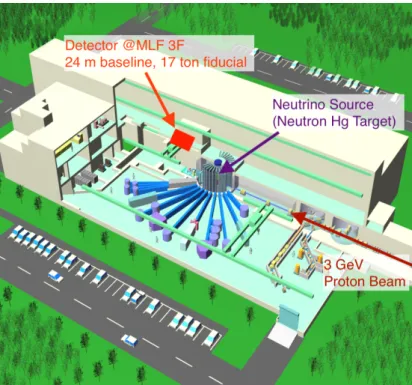
inverse beta decay reaction is an identical method with LSND experiment, and fol-lowing this scheme with improved detection technique ensure a direct test to the result of LSND observation. The JSNS2(PARC Sterile Neutrino Search at J-PARC Spallation Neutron Source) experiment, proposed in 2013 [10], is designed to search for the existence of neutrino oscillations indicated by LSND experiment at the Material and Life science experimental Facility (MLF) in J-PARC. The facility provides an intense neutrino beam from µDAR thanks to the high power and short pulsed proton beam from the Rapid Cycling Synchrotron (RCS) and a spallation neutron target in the MLF. The experiment uses a Gadolinium (Gd) liquid scin-tillator (Gd-LS) detector placed at 24 m away from the mercury target. Both the beam and the detector contribute to detection improvement on ¯νµ→ ¯νe oscillation.

In this chapter, details about the experimental setup and the basic concepts of the JSNS2experiment are described.

2.1 Experimental Setup

The JSNS2experiment is held in J-PARC located in Tokai village, Ibaraki prefecture in east Japan. Figure 2.1 exhibits the bird-eyes view photo of the entire J-PARC fa-cilities. The proton beam is accelerated at the Rapid Cycling Synchrotron (RCS) up to 3 GeV, and sent to a spallation neutron target consisting of mercury in the MLF (the central building in the photo). The JSNS2detector is placed at 24 m away from the mercury target in the MLF as shown in Fig. 2.2. The location is the third floor of the MLF building. Figures 2.3-2.5 show the spatial relation between the detector and the mercury target. The vertical distance from the target to the detector is 13.5 m, and the horizontal one is 20 m. The experimental position is a maintenance area for targets in the MLF. Thus, it is needed to move the detector annually in order to avoid a conflict with the facility works in the summer maintenance period (∼ 2 months).

2.1.1 ν¯e detection technique

As described above, the JSNS2detector observes oscillated ¯νevia inverse beta decay

(IBD) interaction on free proton as ¯νe+ p→ e++ n . One of the advantage of ¯νe

de-tection via IBD is that the final state particles, positron and neutron, can be detected 7

(27)

Figure 2.1: The overview of J-PARC facilities.

(28)

2.1. EXPERIMENTAL SETUP 9

Figure 2.3: A drawing of the MLF third floor in the bird-eye’s view. The detector position is pointed as the red box.

Figure 2.4: A cross section of the MLF building in the orthogonal plain to the beam direction [11]. The red shaded area corresponds to the hot cell where the mercury target is placed. The detector position is pointed as the green box.

(29)

20 m 13.5 m JSNS 2 Detector Hg T arget

Figure 2.5: A cross section of the MLF building in the parallel plain to the beam direction [12].

(30)

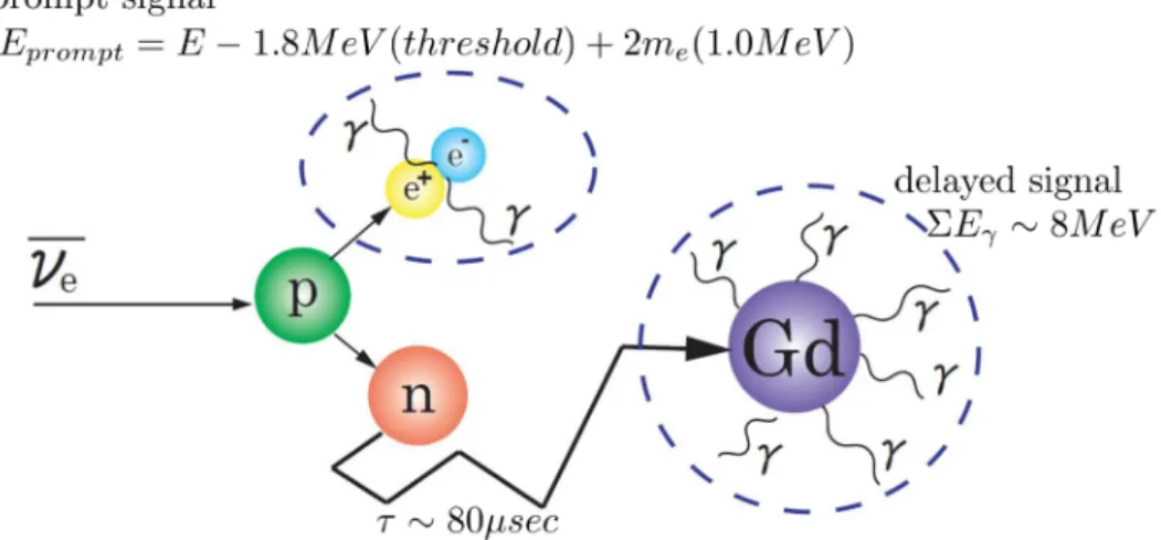
2.1. EXPERIMENTAL SETUP 11 in delayed coincidence method, which significantly suppresses background compared to single event detection. The neutron is captured on nucleus after thermalization,

Figure 2.6: A schematic diagram of delayed coincidence IBD detection used JSNS2experiment.

and emits several gamma rays in a certain time interval from the interaction. The positron immediately generates scintillation light whose amount shows the energy of the anti-electron neutrino. In particular, capture on 155Gd or 157Gd is used in JSNS2case. The schematic of ths process is illustrated in Fig. 2.6. Compared to hy-drogen capture used in LSND experiment, Gd capture has the following advantages:

• large capture cross section: 61 kbarn for thermal neutron (0.0253 eV) on155_Gd,

and 254 kbarn on157Gd.

• total gamma rays energy from thermal neutron capture is roughly 8 MeV,

which exceeds the endpoint energy of environmental gamma ray background;

∼ 2.6 MeV from208_{Tl (c.f., capture on hydrogen: 2.2 MeV).}

• neutron capture time on Gd ∼ 30 µs is shorter than hydrogen capture time ∼

200 µs .

Therefore, the Gd-LS is a quite strong tool for eliminating the accidental background by detecting both positron as a prompt signal and gamma rays from neutron capture on Gd as a delayed signal.

The cross section of the IBD interaction is approximately written down based on the approximation in zeroth order of 1/M from Vogel et at. [13] as a function of neutrino energy Eν: σIBD(Eν) = 0.0952 ( Ee+p_e+ 1 MeV2 ) × 10−42 cm2, (2.1) where Ee+ and p_e+ are the positron energy and the momentum in a unit of MeV, respectively.The positron energy can be approximated by

Ee+ ∼ E_ν+ (M_p− M_n). (2.2)

Therefore, it can be said that the positron keeps the energy information of ¯νe .

As neutrino oscillation distorts neutrino energy spectrum depending on ∆m2, the observed positron energy spectrum also well reflects the oscillation information.

(31)

2.1.2 Detector design

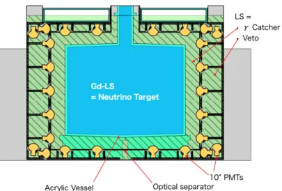
Figure 2.7 shows a schematic of the detector design and structure for the JSNS2_experiment. The JSNS2detector consists of 17 tons Gd-LS contained in an inner acrylic vessel,

and ∼33 tons Gd unloaded liquid scintillator (LS) in the space between the acrylic

vessel and an outer stainless steel tank. The LS layer is separated into two diﬀerent functional layers by optical separators and forms two independent detector volumes in the one detector. The region inside of the optical separator, called ”inner detec-tor”, consists of 17 tons Gd-LS and 25 cm thick LS layer surrounding the Gd-LS volume. The outer layer, called ”veto layer”, has a function to detect cosmic ray induced particles coming into the detector, e.g., cosmic µ . Scintillation light from the inner and veto layers is observed by 10-inch photomultiplier tube (PMT), Hama-matsu R7081: 96 PMTs are mounted in the inner detector and 24 PMTs cover the veto layer. The surfaces in the veto layer carefully covered with reflection material to improve scintillation light collection by the PMTs. The details about R&D for the detector components are described in the later chapter.

Figure 2.7: A schematic view of the JSNS2detector.

2.1.3 Shield

The shield is laid right below the detector in order to suppress gamma ray back-ground.Figure 2.8 shows a photo of the shield before detector installation. It consists of lead bricks and iron plates. The dimension of iron shield is 6 m width × 9 m length × 44 mm thickness. Note that the long side of the iron shield is along the beam direction. On the iron shield, two round-shape lead shield layers are con-structed using about 1500 lead bricks which has 10 cm width, 20 cm length and 5 cm thickness. The radius of them is 1.6 m and 2.5 m, respectively, which means that the Gd-LS region is fully covered with most thick part of the shield (10 cm lead + 4.4 cm iron).

(32)

2.1. EXPERIMENTAL SETUP 13

Figure 2.8: A photo of the shield below the JSNS2_detector.

2.1.4 Annual Operation for Experiment

As mentioned above, the JSNS2_{experiment has to be moved from the MLF building} during the maintenance period of J-PARC in summer. Besides that, Japanese fire law requires that detector contains no flammable materials (= the Gd-LS and the LS) outside of the MLF. Therefore, the following operations (illustrated in figure 2.9) is needed as well as a slow control and data acquisition monitoring during data taking periods.

1. The empty detector is transported from the storage building (HENDEL) to the MLF, and we fill the detector with Gd-LS/LS at the first floor of the MLF from ISO (International Organization for Standardization) tanks, the external storage container.

2. The filled detector is transferred to the experimental position on the 3rd floor of the MLF using a 130-ton crane. The shields consisting of lead and iron beneath the detector is fully laid before this transportation.

3. Data taking launches and is going on until the end of the MLF beam operation (amount to 5000 hours).

4. After the data taking, the detector is moved back the first floor again. The Gd-LS/LS is extracted to each ISO tank, and the empty detector is transported to the HENDEL building for storage until the next beam time.

5. The ISO tanks containing the Gd-LS/LS are stored and managed by Nichiriku company in Kawasaki city.

The ISO tank for Gd-LS/LS storage (shown in figure 2.10) is a container sat-isfying the ISO international standard for liquid storage and transportation, whose inner surface in contact with the Gd-LS/LS is made of stainless steel (SUS316L). Impurity removal and passivation of the stainless steel surface was done by acid

(33)

Figure 2.9: The detector and LS operation during the experiment throughout a year [9].

wash. An examination for an eﬀect of metal surface on the Gd-LS is described in the next chapter. The ISO tank has a capacity of 21 kL so that we uses two tanks for the LS and one tank for the Gd-LS storage.

Figure 2.10: A cut model of an ISO tank with the dimensions labeled [14].

2.2 Decay at Rest Neutrino Beam

The J-PARC MLF is the best suited facility to search for neutrino oscillations using neutrinos from stopped muon decay in the mass range ∆m2 ∼ eV2 for the following reasons:

1. High beam power (1 MW)

2. Suppression of µ− free decay through absorption by the mercury target 3. A low duty factor, pulsed beam which enables elimination of decay-in-flight

components and separation of µDAR from other background sources. The resulting νe, ¯νe have well-defined spectra and known cross sections.

(34)

2.2. DECAY AT REST NEUTRINO BEAM 15

Figure 2.11: A schematic drawing of the J-PARC spallation neutron source [10].

In this section, the details about beam facility and their advantages for the JSNS2experiment mentioned above is explained.

2.2.0.1 The RCS beam and the target

The RCS accelerates protons up to 3 GeV, and periodically sends them to the MLF target in 25 Hz, which corresponds to 40 ms time interval from the previous beam spill. Each spill of beam bunch consists of 100 ns width double pulse with 540 ns interval between them, and the design value of proton intensity is 0.33 mA (1 MW). The 1 MW beam provides 3.8×1022 protons-on-target (POT) during 5000 hours / year operation (i.e. 4.5×108 _{spills are provided during one year).}

Figure 2.11 shows a schematic drawing of the J-PARC spallation neutron source. As a result of mercury spallation via interaction with 3 GeV protons, plenty of hadrons including pion and kaon as well as neutron are produced. The mesons decay and generates neutrinos. The target are surrounded by cooling pipes, beryl-lium reflectors and steel shielding. In addition, there are cryogenic liquid hydrogen moderators located at the top and bottom of the target for neutron beamlines.

The proton beam sent from the RCS enters beamline in the MLF, and collides on the mercury target after passing through a carbon target for µ beamlines. The beam loss due to collision with the carbon target is less than 5%. Figure 2.12 show a 3D model of the mercury target, which has dimensions of 54 cm in width by 19 cm in height by 210 cm in length. The target material, mercury, is encapsulated within multiple wall structure made of stainless steel, and constantly circulated at a rate of 154 kg/sec for cooling.

2.2.0.2 Neutrino beam

The neutrino beam generated in the mercury target has unique timing structure because of the short pulsed beam and lifetime of mother particle of each neutrino. The beam neutrinos can be qualitatively categorized as follows:

(35)

Figure 2.12: A schematic drawing of the mercury target in the J-PARC MLF [10].

• on-bunch: neutrinos produced within 1 µs with respect to the beam collision

timing (mainly π, K decay),

• oﬀ-bunch: neutrinos produced 1 µs after the beam collision timing (mainly µDAR).

Quantitatively, MC simulation for beam neutrino flux estimation was performed in the following sequences:

1. Secondary particle production by 3 GeV protons

The interaction of 3 GeV proton beam with the mercury target and beam-line components has been simulated using FLUKA [18] and QGSP-BERT (in Geant4 [19]) hadron interaction simulation packages [10].

2. π± interactions and decay

The charged pion (π+ and π−) produced in the target deposits its kinetic energy to materials via ionization. The charge exchange reaction (π+n→ π0p

or π−p → π0n, then π0 → γγ) decreases the number of the charged pions.

The behavior of charged pions diﬀer depending on their sign of charge: π+ stops and decays with its lifetime in vacuum (26 ns) because it is repulsed by positive chrge of neucleus. On the other hand, the survived π−are absorbed by forming a π-mesic atoms. π decay-in-flight is highly suppressed to∼ 8 × 10−3 of the produced π±.

3. µ± absorption and decay

µ+ decays in the reaction µ+ → e+νeν¯µ. Because of the muon lifetime and

energy loss process, the decay-in-flight is negligible. µ− is captured by nuclei by forming a mu-mesic atom, and eventually produces νµ with an endpoint

energy of 105 MeV. The absorption rate depends on the atomic number of nucleus, i.e., the eﬀect becomes larger in heavier nuclei. The total rate of µ− capture on nucleus have been measured in terms of eﬀective muon lifetime [20]. Figure 2.13 shows the timing profile of neutrinos generated in the mercury target obtained from the MC simulation. The black square pulse corresponds to the proton