GLOBAL CONVERGENCE RESULTS OF A NEW THREE-TERM MEMORY GRADIENT METHOD

(1)

2004, Vol. 47, No. 2, 63-72

GLOBAL CONVERGENCE RESULTS OF A NEW THREE-TERM MEMORY GRADIENT METHOD

Sun Qingying Liu Xinhai University of Petroleum

(Received March 5, 2002; Received January 7, 2004)

Abstract In this paper, a new class of three-term memory gradient methods with Armijo-like step size rule for unconstrained optimization is presented. Global convergence properties of the new methods are discussed without assuming that the sequence{xk}of iterates is bounded. Moreover, it is shown that, when f(x) is pseudo-convex (quasi-convex) function, this new method has strong convergence results. Combining FR, PR, HS methods with our new method, FR, PR, HS methods are modiﬁed to have global convergence property. Numerical results show that the new algorithms are eﬃcient.

Keywords: Nonlinear programming, three-terms memory gradient method, Armijo-like step size rule, convergence, numerical experiment

1. Introduction

Consider the following unconstrained problem

min{f(x) :x∈Rⁿ}, (1)

where f :Rⁿ→R is a continuously diﬀerentiable function.

In [2], the memory gradient algorithm for problem (1) was ﬁrst presented. Compared with the ordinary gradient method, this algorithm has the advantage of high speed. Cragg and Levy [1] made a generalization of the memory gradient algorithm and presented a method called the super-memory gradient algorithm which from numerical experience has been shown to be much more rapidly convergent, in general, than the memory gradient algorithm.

In this paper, we consider a new three-terms memory gradient method for problem (1) whose search directions are deﬁned by

d_k =−∇f(x_k) +β_kd_k−1+α_kd_k−2, (2) and

x_k+1 =x_k+λ_kd_k, (3)

whereβ_kandα_kare parameters andλ_kis a step-size obtained by means of a one-dimensional search. Conditions are given on β_k and α_k to ensure thatd_k is a suﬃcient descent direction at the point x_k of iterate. Global convergence properties of the new class of three terms memory gradient methods with Armijo-like step size rule are discussed without assuming that the sequence {x_k} of iterates is bounded. Moreover, it is shown that, when f(x) is pseudo-convex (quasi-convex) function, this new method has strong convergence results.

(2)

Combining FR, PR, HS methods with our new method, FR, PR, HS methods are modiﬁed to have global convergence property. Numerical results show that the new algorithms are eﬃcient.

In Section 2, we present a new method. We start the convergence analysis of the new method in Section 3. The convergence properties for generalized convex functions are discussed in Section 4. Finally, a detailed list of the test problems that we have used is given in Section 5.

2. The New Three-term Memory Gradient Algorithm

Consider the three-term memory gradient method (2) and (3). LetS_k =−∇f(x_k) +β_kd_k−1. In order to ensure that d_k is a suﬃcient descent direction, we assume that





∇f(x_k)^T∇f(x_k)>|β_k∇f(x_k)^Td_k−1|,

∇f(x_k)^TS_k ≥(1 +^k₁)|β_k| · ∇f(x_k) · d_k−1 (4) and





|∇f(x_k)^TS_k|>|α_k∇f(x_k)^Td_k−2|,

|∇f(x_k)^Td_k| ≥(1 +^k₂)|α_k| · ∇f(x_k) · d_k−2 (5) where ^k₁ >0,^k₂ >0 are parameters.

Condition (4) plays a vital role in choosing β_k, and a new choice for β_k is given by β_k∈[−β

k(^k₁), β_k(^k₁)], (6)

β_k(^k₁) = 1

(1 +^k₁) + cosθ_k · ∇f(x_k)

d_k−1 , (7) βk(^k₁) = 1

(1 +^k₁)−cosθ_k ·∇f(x_k)

d_k−1 , (8) where θ_k is the angle between ∇f(x_k) and d_k−1.

Condition (5) plays a vital role in choosing α_k, and a new choice for α_k is given by α_k ∈[−α_k(^k₁,^k₂), α_k(^k₁,^k₂)], (9) α_k(^k₁,^k₂) = 1 +^k₁

2 +^k₁ · 1

(1 +^k₂) + cosθ_k · ∇f(x_k)

d_k−2 , (10) α_k(^k₁,^k₂) = 1 +^k₁

2 +^k₁ · 1

(1 +^k₂)−cosθ_k · ∇f(x_k)

d_k−2 , (11) where θ_k is the angle between∇f(x_k) and d_k−2.

The new three-terms memory gradient algorithm (NTMG):

Data: ∀ x₁ ∈Rⁿ, d₀ = 0, ⁰₁ >0, ⁰₂ >0, µ₁, µ₂ ∈(0,1) and µ₁ ≤µ₂, γ₁, γ₂ >0,γ₂ <1.

Step1: Compute∇f(x₁), if ∇f(x₁) = 0, and x₁ is a stationary point of (1), stop; else set d₁ =−∇f(x₁), k := 1, and go to step2.

Step2: x_k+1 =x_k+λ_kd_k, the step size λ_k is chosen so that

f(x_k+λ_kd_k)≤f(x_k) +µ₁λ_k∇f(x_k)^Td_k, (12)

(3)

and

λ_k≥γ₁ or λ_k ≥γ₂λ^∗_k >0, (13) where λ^∗_k satisﬁes

f(x_k+λ^∗_kd_k)> f(x_k) +µ₂λ^∗_k∇f(x_k)^Td_k, (14)

Step3: Compute∇f(x_k+1). if∇f(x_k+1)= 0, and x_k+1 is a stationary point of (1), stop;

else let k: =k+ 1, ^k₁ ≥ ⁰₁, ^k₂ ≥ ⁰₂, and go to step4.

Step4: Letd_k =−∇f(x_k) +β_kd_k−1+α_kd_k−2, where β_k∈[−β

k(^k₁), β_k(^k₁)],α_k ∈[−α_k(^k₁,^k₂), α_k(^k₁,^k₂)], go to step 2.

Remark We can give the new choice of the parameter β_k: β_k= argmin{|β−β_k^{F R}||β ∈[−β

k(^k₁), β_k(^k₁)]}; β_k= argmin{|β−β_k^{P R}||β ∈[−β

k(^k₁), β_k(^k₁)]}; β_k= argmin{|β−β_k^HS||β ∈[−β

k(^k₁), β_k(^k₁)]};

where β_k^{F R} = g_k ²/g_k−1 ² (Fletcher-Reeves), β_k^{P R} = g_k^T(g_k −g_k−1)/g_k−1 ² (Polak- Ribiere),β_k^HS = (g_k^T(g_k−g_k−1))/d^T_k−1(g_k−g_k−1) (Hestenes-Stiefel), and three classes of new methods are established, denoted by NTFR, NTPR, NTHS, respectively. In particular, we can takeα_k = 0 in NTMG, NTFR, NTPR, NTHS methods, and four classes of new methods are established, denoted by NCG, NFR, NPR, NHS, respectively.

Lemma 1 Ifx_k is not a stationary point for problem (1), thend_k ≤c₁∇f(x_k), where c₁ = 1 +¹₀

1 +¹₀

2.

Proof. It follows from the deﬁnition of d_k.

Lemma 2 If x_k is not a stationary point for problem (1), then d_k is a descent direction, i.e. ∇f(x_k)^Td_k ≤ −c₂· ∇f(x_k)², where c₂ = ¹⁺₂₊⁰¹₀

1 · ¹⁺₂₊⁰²0 2.

Proof. For k = 1, it is clear that d₁ = −∇f(x₁) is a descent direction. For k ≥ 2, by using assumption (4) and the deﬁnition of S_k, we have

∇f(x_k)^TS_k = −∇f(x_k)²+β_k· ∇f(x_k)^Td_k−1

≤ −∇f(x_k)²+|β_k· ∇f(x_k)^Td_k−1|

≤ −∇f(x_k)²+∇f(x_k)²

= 0.

It follows from (4) that

∇f(x_k)^TS_k ≤ −∇f(x_k)²+|β_k· ∇f(x_k)^Td_k−1|

≤ −∇f(x_k)²+ 1

1 +^k₁|∇f(x_k)^TS_k|. The above inequality and|∇f(x_k)^TS_k|=−∇f(x_k)^TS_k imply that

∇f(x_k)^TS_k ≤ −1 +^k₁

2 +^k₁ · ∇f(x_k)². (15)

(4)

Since for k = 2, d₂ is identical with s₂, the result follows from equation (15). For k ≥3, it follows from (5) and the deﬁnition of d_k and (15) that

∇f(x_k)^Td_k ≤ −1 +^k₂

2 +^k₂ · |∇f(x_k)^TS_k| ≤ −1 +^k₁

2 +^k₁ · 1 +^k₂

2 +^k₂ · ∇f(x_k)². By using ¹⁺₂₊^k¹_k

1 ≥ ¹⁺₂₊⁰¹0

1, for ^k₁ ≥ ⁰₁ and ¹⁺₂₊^k²_k

2 ≥ ¹⁺₂₊⁰²0

2, for ^k₂ ≥ ⁰₂, we obtain that

∇f(x_k)^Td_k ≤ −¹⁺₂₊^k¹k

1 · ¹⁺₂₊^k²k

2 · ∇f(x_k)². 3. Convergence Analysis

Throughout this paper, let{x_k}denote the sequence generated by (NTMG). If∇f(x_k) = 0 for a ﬁnite integer k, x_k is a stationary point of (1). In what follows, we assume that (NTMG) generates an inﬁnite sequence. We now present our global convergence results.

Theorem 1 Suppose that f(x)∈C¹. Then:

(i) either f(x_k)→ −∞ or lim inf_k→∞∇f(x_k)= 0;

(ii) either f(x_k)→ −∞ or lim_k→∞∇f(x_k)= 0, if ∇f is uniformly continuous on Rⁿ . Proof. Since for all k, ∇f(x_k)^Td_k < 0, we havef(x_k+1) < f(x_k), which implies that {f(x_k)} is a monotonically decreasing sequence. If f(x_k) → −∞, then we complete the proof. Therefore, in the following discussion, we assume that {f(x_k)} is a bounded set.

Suppose (i) is not true. Then, there exists ε >0 such that, for all k,

∇f(x_k)≥ε. (16) It follows from Lemma 2, (12) and (16) that

f(x_k+ 1)−f(x_k)≤µ₁λ_k∇f(x_k)^Td_k ≤ −c₂λ_kµ₁∇f(x_k)² ≤ −c₂λ_kµ₁ε∇f(x_k). (17) The above inequality and the boundedness of {f(x_k)} imply that

∞ k=1

λ_k∇f(x_k)<+∞. (18)

It follows from Lemma 1 and (2) that, for all k,

x_k+1−x_k=λ_kd_k ≤c₁λ_k∇f(x_k).

The above inequalities and (18) yield ^∞_k=1x_k+1−x_k < +∞, which yields that{x_k} is convergent, say to a point x_∗. From (16), (18), we have

k→∞lim λ_k = 0. (19)

It follows from Lemma 1, the convergence of {x_k} and f(x) ∈ C¹ that {d_k} is bounded.

Without loss of generality, we may assume that there exists an index set K ⊂ {1,2, ...} such that lim_{k→∞,k∈K}d_k = d_∗. It follows from (13) and (19) that, when k(k ∈ K) is large enough, we haveλ_k < γ₁, and hence it follows from (13) that, λ_k ≥γ₂λ^∗_k, where λ^∗_k satisﬁes (14), i.e. f(x_k+λ^∗_kd_k)−f(x_k)/λ^∗_k ≥µ₂λ^∗_k∇f(x_k)^Td_k. Taking the limit for k ∈K, we have

∇f(x_∗)^Td_∗ ≥µ₂∇f(x_∗)^Td_∗. (20)

(5)

By using (20) and µ₂ ∈(0,1) , we obtain that

∇f(x_∗)^Td_∗ = 0. (21) It follows from Lemma 2 and (21) that ∇f(x_∗) = 0 , which contradicts (16). This completes the proof of (i).

Suppose that there exist an inﬁnite index set K₁ ⊂ {1,2, ...} and a positive scalar ε >0 such that, for all k∈K₁,

∇f(x_k)> ε. (22)

It follows from Lemma 2 and (12)that

f(x_k)−f(x_k+1)≥ −µ₁λ_k∇f(x_k)^Td_k ≥c₂λ_kµ₁∇f(x_k)². (23) By using (22) and (23), we obtain that λ_k ≤µ⁻¹₁ ⁻²c⁻¹₂ (f(x_k)−f(x_k+1), ∀k∈K₁.

The boundedness of {f(x_k)} and the monotonically decreasing property imply that {f(x_k)} is convergent. Thus,

lim sup

k→∞,k∈K1

λ_k≤ lim sup

k→∞,k∈K1

µ⁻¹₁ ⁻²c⁻¹₂ (f(x_k)−f(x_k+1), which yields that

lim sup

k→∞,k∈K1

λ_k = 0. (24)

It follows from (22) and (23) thatλ_k∇f(x_k)≤µ⁻¹₁ ⁻¹c⁻¹₂ (f(x_k)−f(x_k+1)), and lim sup_{k→∞,k∈K}₁λ_k∇f(x_k)≤lim sup_{k→∞,k∈K}₁µ₁⁻¹⁻¹c⁻¹₂ (f(x_k)−f(x_k+1)). Hence,

lim sup

k→∞,k∈K1

λ_k∇f(x_k) = 0. (25)

It follows from Lemma 1 and (25) that lim sup

k→∞,k∈K1

λ_kd_k ≤ lim sup

k→∞,k∈K1

c₁λ_k∇f(x_k). i.e.

lim sup

k→∞,k∈K1

λ_kd_k= 0. (26)

It follows from (24) that, when k(k ∈ K₁) is large enough, we have λ_k < γ₁, and hence it follows from (13) that, λ_k ≥ γ₂λ^∗_k, where λ^∗_k satisﬁes (14). Now set x^∗_k+1 = x_k +λ^∗_kd_k. It follows from (24), (26) and λ_k ≥ γ₂λ^∗_k, ( k ∈ K₁ is large enough) that lim_{k→∞,k∈K}₁λ^∗_k = 0 and lim_{k→∞,k∈K}₁λ^∗_kd_k= 0. Hence, lim_{k→∞,k∈K}₁x^∗_k+1−x_k= 0.

Let ρ^∗_k = ^f(x^∗^k+1^)−f(x^k⁾

λ^∗_k∇f(xk)^Tdk , k ∈K₁, it follows from (14) that

ρ^∗_k < µ₂ <1, k∈K₁. (27) It follows from Lemmas 1, 2 and (22) that

lim sup

k→∞,k∈K1

|ρ^∗_k−1|= lim sup

k→∞,k∈K1

|∇f(ξ_k^∗)^T(λ^∗_kd_k) λ^∗_k∇f(x_k)^Td_k −1|

= lim sup

k→∞,k∈K1

|(∇f(ξ_k^∗)− ∇f(x_k))^Td_k

∇f(x_k)^Td_k | ≤ lim sup

k→∞,k∈K1

∇f(ξ^∗_k)− ∇f(x_k) · d_k

|∇f(x_k)^Td_k|

≤ lim sup

k→∞,k∈K1

∇f(ξ_k^∗)− ∇f(x_k) ·c₁· ∇f(x_k) c₂ · ∇f(x_k)²

≤ lim sup

k→∞,k∈K1

∇f(ξ_k^∗)− ∇f(x_k) ·c₁

c₂ ·ε = 0, (28)

(6)

where ξ_k^∗ =x_k+ϑ_k(x^∗_k+1−x_k),0< ϑ_k <1, k ∈K₁.

Hence (28) establishes that ρ^∗_k ≥ µ₂ for all k ∈K₁ suﬃciently large. This is the desired contradiction because (27) guarantees thatρ^∗_k < µ₂. This yields (ii).

4. Convergence Properties for Generalized Convex Functions

In this section, we discuss the convergence properties of (NTMG) for generalized convex functions. As shown in the following, parameters ^k₁,^k₂ play an important role in our analysis. We make the following assumption:

(Q) For any integer k,

^k₁ ≥max{⁰₁, 1 +x_k

f(x_k−1)−f(x_k)∇f(x_k)}, ^k₂ ≥max{⁰₂, 1 +x_k

f(x_k−1)−f(x_k)∇f(x_k)}. Thus we have the following results.

Lemma 3 Suppose that (Q) holds and f(x) ∈ C¹. Let λ₀ = sup{λ_k, k = 1,2, ...} and suppose that λ₀ < +∞. If f(x) is a quasi-convex function and the solution set of problem (1) is nonempty, then {x_k} is a bounded sequence, each accumulation point x_∗ of which is a stationary point of problem (1) and lim_k−→∞x_k =x_∗.

Proof. Note that for all x∈Rⁿ and allk,

x_k+1−x² = x_k−x²+ 2(x_k+1−x, x_k−x) +x_k+1−x_k²

= x_k−x²+ 2λ_k(d_k, x_k−x) +λ²_kd_k²

= x_k−x²+ 2λ_k(−∇f(x_k) +β_kd_k−1 +α_kd_k−2, x_k−x) +λ²_kd_k²

≤ x_k−x²+ 2λ_k(∇f(x_k), x−x_k)

+2λ_k|β_k|d_k−1x_k−x+ 2λ_k|α_k|d_k−2x_k−x+λ²_kd_k²

≤ x_k−x²+ 2λ_k(∇f(x_k), x−x_k) +4λ_kf(x_k−1)−f(x_k)

1 +x_k (x_k+x) +λ²_kd_k²

≤ x_k−x²+ 2λ_k(∇f(x_k), x−x_k)

+4λ₀(1 +x)(f(x_k−1)−f(x_k)) +λ²_kd_k². (29) It follows from Lemma 1, Lemma 2 and (12) that

d_k² ≤c²₁∇f(x_k)²; (30)

∇f(x_k)² ≤c⁻¹₂ (−∇f(x_k))^Td_k); (31)

−λ_k∇f(x_k))^Td_k ≤µ⁻¹₁ ((f_k)−f(x_k+1)). (32) By using (29), (30), (31), (32) and the above inequality, we obtain that

x_k+1−x² ≤ x_k−x²+ 2λ_k(∇f(x_k), x−x_k)

+4λ₀(1 +x)(f(x_k−1)−f(x_k)) +λ₀λ_kc²₁c⁻¹₂ (−∇f(x_k)^Td_k)

≤ x_k−x²+ 2λ_k(∇f(x_k), x−x_k)

+4λ₀(1 +x)(f(x_k−1)−f(x_k)) +λ₀c²₁c⁻¹₂ µ⁻¹₁ (f(x_k)−f(x_k−1))).

= x_k−x²+ 2λ_k(∇f(x_k), x−x_k)

+m₁(x)(f(x_k−1)−f(x_k)) +m₂(f(x_k)−f(x_k−1))), (33)

(7)

where m₁(x) = 4λ₀(1 +x), m₂ =λ₀µ⁻¹₁ c²₁c⁻¹₂ .

Because the solution set of problem (1) is nonempty, we can choose y ∈ Rⁿ satisfying f(y)≤f(x_k). Since f(x) is a quasi-convex function, we have

(∇f(x_k), y−x_k)≤0. (34)

It follows from (33), (34) that

x_k+1−y²+m₁(y)f(x_k) +m₂f(x_k+1)≤ x_k−y² +m₁(y)f(x_k−1) +m₂f(x_k) which implies the sequence{x_k−y²+m₁(y)f(x_k−1) +m₂f(x_k)}is descent. Since we have assumed that the solution set of problem (1) is nonempty, and so inf{f(x_k) :k = 1,2, ...}>

−∞ both sequence {f(x_k)} and {x_k−y²+m₁(y)f(x_k−1) +m₂f(x_k)} are bounded from below and converge. Therefore, the sequence {x_k−y²} converges and {x_k} is bounded.

This implies that {x_k} has an accumulation point x_∗ and that there exists an index set K₁ ⊂ {1,2, ...} such that lim_{k→∞,k∈K}₁x_k = x_∗, and lim_{k→∞,k∈K}₁f(x_k) = f(x_∗). It follows from the above equation and the fact{f(x_k)}is a monotonically decreasing sequence implies lim_{k→∞,k∈K}₁f(x_k−1) =f(x_∗). Therefore, we have

k→∞lim {x_k−x_∗²+m₁(x_∗)f(x_k−1) +m₂f(x_k)}

= lim

k→∞,k∈K1{x_k−x_∗²+m₁(x_∗)f(x_k−1) +m₂f(x_k)}

= [m₁(x_∗) +m₂]f(x_∗),

which implies lim_k→∞x_k =x_∗. From Theorem 1 the limit pointx_∗ is a stationary point of problem (1).

Theorem 2 Suppose that (Q) holds and f(x) ∈ C¹ . Let λ₀ = sup{λ_k, k = 1,2, ...} and suppose that λ₀ <+∞. If f(x) is a pseudo-convex function, then:

(i) {x_k}is a bounded sequence if and only if the solution set of problem (1) is nonempty;

(ii) lim_k→∞f(x_k) = inf{f(x) :x∈Rⁿ};

(iii) If the solution set of problem (1) is nonempty, then any accumulation point x_∗ of {x_k}is an optimal solution of problem (1) and lim_k→∞x_k =x_∗.

Proof. Since f(x) is pseudo-convex, it is quasi-convex and a stationary point of problem (1) is also an optimal solution of problem (1).

First, we will show part (i). If {x_k}is a bounded sequence, then it follows from Theorem 1 that there exists an index setK₂ ⊂ {1,2, ...}and a pointx_∗ ∈Rⁿsuch that lim_{k→∞,k∈K}₁x_k = x_∗, and x_∗ is a stationary point of problem (1), and is also an optimal solution of problem (1). Conversely, if the solution set of problem (1) is nonempty, then it follows from Lemma 3 that {x_k} is a bounded sequence.

Next, we will prove (ii). We prove this conclusion by the following three cases (a), (b), (c).

(a) lim_k→∞f(x_k) = inf{f(x) : k = 1,2, ...}=−∞; It follows from {f(x_k)} is a descent sequence, and lim_k→∞f(x_k) = inf{f(x) :k = 1,2, ...} ≥inf{f(x) :x∈Rⁿ}.

(b) {x_k}is bounded: It follows from (i) of this theorem that the solution of problem (1) is nonempty, and there exists an index set K₃ ⊂ {1,2, ...} and a point x_∗ ∈ Rⁿ such that lim_{k→∞,k∈K}₁x_k =x_∗,it follows from Theorem 1 thatx_∗ is a stationary point of problem (1), and is also an optimal solution of problem (1).

(8)

(c) inf{f(x) : k = 1,2, ...} > −∞; and {x_k} is unbounded: Suppose that there exists

¯

x ∈ Rⁿ, ε > 0, and k₁ such that for all k ≥k₁, f(x_k) > f(¯x) +ε. Since f(x) is a pseudo- convex function, we have (∇f(x_k),x¯− x_k) ≤ 0, for all k ≥ k₁. Setting x = ¯x in (33) that

x_k+1−x¯² +m₁(¯x)f(x_k) +m₂f(x_k−1)≤ x_k−x¯²+m₁(¯x)f(x_k−1) +m₂f(x_k), which implies the sequence {x_k−x¯² +m₁(¯x)f(x_k−1) +m₂f(x_k)} is descent. Since we have assumed that inf{f(x) :k = 1,2, ...}>−∞; both sequence{f(x_k)} and {x_k−x¯²+ m₁(¯x)f(x_k−1) +m₂f(x_k)} are bounded from below and converge. Therefore, the sequence {x_k−x¯²}converges and {x_k} is bounded, which contradicts our assumption.

(iii) immediately follows from Lemma 3.

Corollary 1 Suppose that (Q) holds and f(x) ∈C¹ . Let λ₀ = {sup{λ_k, k = 1,2, ...} and suppose that λ₀ <+∞. If f(x) is a convex function, then:

(i) {x_k}is a bounded sequence if and only if the solution set of problem (1) is nonempty;

(ii) lim_k→∞f(x_k) = inf{f(x) :x∈Rⁿ}.

(iii) If the solution set of problem (1) is nonempty , then any accumulation point x_∗ of {x_k}is an optimal solution of problem (1) and lim_k→∞x_k =x_∗.

Proof. Since f(x) is convex, it is pseudo-convex. It immediately follows from Theorem 2.

Corollary 2 Suppose that (Q) holds and f(x) ∈ C¹. Let λ₀ = sup{λ_k, k = 1,2, ...} and suppose that λ₀ < +∞. If f(x₎ is a quasi-convex function, then either the solution set of problem (1) is empty or any accumulation point x_∗ of {x_k} is a stationary point of problem (1) and lim_k→∞x_k =x_∗.

Proof. It immediately follows from Lemma 3.

Note that Wei and Jiang [4] has obtained a similar result to Corollary 1 for gradient descent method with convex function.

5. Numerical Experiments

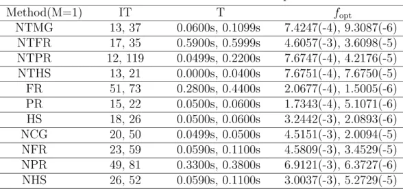
We choose three numerical examples from [3], and report some numerical results by using the new methods in this paper. We take ⁰₁ = 0.067, ⁰₂ = 3, α_k = α_k(^k₁,^k₂), µ₁ = µ₂ = µ= 0.25, β = 1/2.9, γ = 1, ( NTMG β_k =β_k(^k₁).) We denote by ”IT” the number of iterations, by ”f_opt” the objective function value at the solution, by ”T” computational time, by ”3.6461(-3)” ”3.6461 ” etc. The following is the numerical results.

Example 1

f(x) = 10(x²₁ −x₂)²+ (1−x₁)²+ 9(x₄−x²₃)²+ (1−x₃)² +10.1((x₂−1)²+ (x₄−1)²) + 19.8(x₂−1)(x₄−1) x₁ = (−3,−1,−3,−1)^T; x_opt = (1,1,1,1);f(x_opt) = 0.

∇f(x_k) ≤10⁻¹, 10⁻² Example 2 f(x) = ^N/2_i=1[(x_2i −x²_2i−1)²+ (1−x_2i−1)²];

x₁ = (−1.2,1,−1.2,1, ...,−1.2,1)^T;−x_opt = (1,1, ...,1);f(x_opt) = 0.

∇f(x_k) ≤10⁻¹, 10⁻², N=120

(9)

Table 1: Numerical results of example 1

Method(M=1) IT T f_opt

NTMG 13, 37 0.0600s, 0.1099s 7.4247(-4), 9.3087(-6) NTFR 17, 35 0.5900s, 0.5999s 4.6057(-3), 3.6098(-5) NTPR 12, 119 0.0499s, 0.2200s 7.6747(-4), 4.2176(-5) NTHS 13, 21 0.0000s, 0.0400s 7.6751(-4), 7.6750(-5) FR 51, 73 0.2800s, 0.4400s 2.0677(-4), 1.5005(-6) PR 15, 22 0.0500s, 0.0600s 1.7343(-4), 5.1071(-6) HS 18, 26 0.0500s, 0.0600s 3.2442(-3), 2.0893(-6) NCG 20, 50 0.0499s, 0.0500s 4.5151(-3), 2.0094(-5) NFR 23, 59 0.0590s, 0.1100s 4.5809(-3), 3.4529(-5) NPR 49, 81 0.3300s, 0.3800s 6.9121(-3), 6.3727(-6) NHS 26, 52 0.0590s, 0.1100s 3.0037(-3), 5.2729(-5)

NTMG 8, 11 14.6599s, 19.5000s 5.8984(-3), 7.9117(-6) NTFR 8, 11 14.6700s, 19.3800s 6.1615(-4), 1.3811(-5) NTPR 9, 14 16.2600s, 23.5600s 1.6195(-3), 6.9608(-5) NTHS 9, 25 16.1000s, 39.6499s 4.7874(-3), 1.4845(-5) FR 13, 19 39.2699s, 56.3499s 2.0765(-3), 1.4603(-5) PR 9, 11 26.4200s, 32.1299s 8.0624(-3), 4.1389(-4) HS 9, 11 26.4800s, 32.3933s 1.1136(-3), 8.9999(-5) NCG 12, 16 19.0600s, 24.9900s 1.7409(-2), 4.2189(-4) NFR 12, 19 35.3099s, 55.8100s 3.2288(-2), 1.7576(-4) NPR 14, 15 41.0899s, 43.8800 1.3835(-3), 1.2374(-5) NHS 17, 23 49.8799s, 67.3900s 2.3040(-2), 1.3199(-5)

(10)

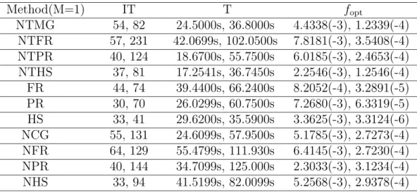
Example 3

f(x) = ^N/4_i=1[(x_4i−1+ 10x_4i−2)²+ 5(x_4i−1−x_4i)² + (x_4i−2−2x_4i−1)²+ 10(x_4i−3 −x_4i)²];

x₁ = (3,−1,0,−3,−3,−1,0,−3, ...,−3,−1,0,3)^T;−x_opt = (0,0, ...,0); f(x_opt) = 0.

∇f(x_k) ≤10⁻¹, 10⁻², N=60

NTMG 54, 82 24.5000s, 36.8000s 4.4338(-3), 1.2339(-4) NTFR 57, 231 42.0699s, 102.0500s 7.8181(-3), 3.5408(-4) NTPR 40, 124 18.6700s, 55.7500s 6.0185(-3), 2.4653(-4) NTHS 37, 81 17.2541s, 36.7450s 2.2546(-3), 1.2546(-4) FR 44, 74 39.4400s, 66.2400s 8.2052(-4), 3.2891(-5) PR 30, 70 26.0299s, 60.7500s 7.2680(-3), 6.3319(-5) HS 33, 41 29.6200s, 35.5900s 3.3625(-3), 3.3124(-6) NCG 55, 131 24.6099s, 57.9500s 5.1785(-3), 2.7273(-4) NFR 64, 129 55.4799s, 111.930s 6.4145(-3), 2.7230(-4) NPR 40, 144 34.7099s, 125.000s 2.3033(-3), 3.1234(-4) NHS 33, 94 41.5199s, 82.0099s 5.2568(-3), 2.9378(-4)

The numerical results indicate the proposed new methods have performance superior to the classical FR, PR, HS algorithms with Armijo-like step size rule, especially in the total amount of computational time. Moreover, the new methods are stable, and attractive for large-scale optimization problems.

Acknowledgment

The author wishes to express his thanks to referees for their very helpful comments.

References

[1] E. E. Cragg and A. V. Levy: Study on supermemory gradient method for the minimization of functions. Journal of Optimization Theory and Applications, 4 (1969) 191-205.

[2] A. Miele and J. W. Cantrell: Study on a memory gradient method for the minimization of functions. Journal of Optimization Theory and Applications,3 (1969) 457-470.

[3] D. Touati-Ahmed and C. Storey: Eﬃcient hybrid conjugate gradient techniques.Jour- nal of Optimization Theory and Applications, 64 (1990) 379-397.

[4] Z. Wei, L. Qi, and H. Jiang: Some convergence properties of descent methods.Journal of Optimization Theory and Applications,95 (1997) 177-188.

Sun Qingying

Depart. of Applied Maths University of Petroleum

Dongying, 257061, P.R.CHINA E-mail: sunqingying01@163.com