Research and design on a control system for a disk-type flying robot with multiple rotors
Ikuo Yamamoto
∗, Rui Zhu
∗, James F. Whidborne
†, Aryeh Marks
†∗Graduate School of Engineering, Nagasaki University, Japan
†School of Engineering, Cranfield University, UK Abstract—This paper describes the development of a disk-type
flying robot with multiple rotors for use as an aerial observation platform. Models for the system are presented. A control system based on the optimal linear quadratic regulator is proposed.
The controller is tested on the simulation model and shown to provide tracking of the reference trajectory and robustness against environmental disturbances.
I. INTRODUCTION
Following a natural disaster, such as an earthquake, ty- phoon or tsunami, a quick response is required to keep utility supply lines open, with electricity being especially important.
For example, if a utility pylon located in a remote moun- tainous or island region is damaged, the disaster area might be surveyed to check damage conditions using a manned helicopter. Flying observations can be carried out with manned operators; however it might not always be practical due to a shortage in skilled operators. Hence a development of unmanned air observation platforms (flying robots) is required for such circumstances. However, the actuation mechanism for traditional single-rotor rotorcraft is mechanically complicated.
Hence alternative configurations may be preferable.
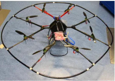
Fig. 1. Disk-type flying robot
One common configuration is the quadrotor [1, for exam- ple] with independently actuated in-line rotors. This can be extended to a multirotor disk-type flying robot configuration as shown in 1 that has been developed by the authors [2].
Modifications to the arms and shape of the flying robot have been made to improve the aerodynamics (see Fig 2) and to protect the rotors in case of impact [3]. Figure 3 shows the robot undergoing a flight test.
In this paper, optimal feedback control is applied to the flying robot that provides excellent tracking performance of the reference trajectory and good robustness against environmental disturbance. In the next section, following a list of modelling assumptions, the model of the flying robot is presented. In Section III, a controller based on the Linear Quadratic Regu- lator (LQR) is presented. In Section IV, the controller design is discussed, analyzed and tested using a simulation based on the model of Section II. Finally, some conclusions are drawn.
(a) Air flow analysis of conven- tional arm
(b) Air flow analysis of modified arm
Fig. 2. Flow around the motor
Fig. 3. Disk-type robot in flight
II. DEVELOPMENT OF MODEL
The control system design and development of modelling flying robot was performed to a 6 DOF motion in dynamic coordinate system and stationary coordinate system. The fol- lowing assumptions are made
• the robot structure is rigid and symmetric,
• the inertia matrix is diagonal,
• ground effect is neglected,
• and the body aerodynamic forces are not included.
The control is assumed to consist of thrusts in and moments about the body axes. In practice these are generated by rotors, so the following assumptions are hence made for the rotors
• the propellers blades are rigid,
• the thrust and torque generated by each motor is the control,
• the rotor Coriolis force are ignored and
• and the motor dynamics are ignored.
The body-fixed frame has the x, y andz axes originating at the center of mass of the vehicle. An inertial coordinate frame is fixed to the Earth and has axes in the conventional North- East-Down arrangement.It is assumed that the Earth is flat and stationary.
A rotation matrix of Tait-Bryan angles can be expressed as
R(φ, θ, ψ) =RφRθRψ (1)
=
" cθcψ cθsψ −sθ
sφsθcψ−cφsψ sφsθsψ+cφcψ sφcθ
cφsθcψ+sφsψ cφsθsψ−sφcψ cφcθ
# (2) wherecθ denotescosθ,sθ denotessinθ, etc.
From Newton’s second law, the time derivative of mo- mentum is equal to the external force and the time derivative of angular momentum is equal to the external moment. The translational equation of motion of the flying robot body axes frame is
"u˙
˙ v
˙ w
#
=−Ω
"u v w
# + 1
m
"Xg Yg
Zg
# + 1
m
"X Y Z
#
, (3)
whereΩis a skew symmetric matrix given by Ω =
"0 −r q
r 0 −p
−q p 0
#
, (4)
Xg,Yg,Zg are the body gravity forces in thex,y,zdirection body axes respectively,X,Y,Z are the rotor thrusts in thex, y,zdirection body axes respectively andmis the body mass.
Expanding (3) gives
"u˙
˙ v
˙ w
#
=
" rv−qw−gsθ+X/m
−ru+pw+gsφcθ+Y /m qu−pv+gcθcφ+Z/m
#
. (5)
Therefore, the velocity of the flying robot in the inertial coordinate system is
"x˙
˙ y
˙ z
#
=R(φ, θ, ψ)
"u v w
#
. (6)
The translational motion in the inertial axes is given by
"x¨
¨ y
¨ z
#
= 1
mR(φ, θ, ψ) "Xg
Yg
Zg
# +
"X Y Z
#!
(7) which simplifies to
"x¨
¨ y
¨ z
#
=
" (sψsφ+cψsθcφ)Z/m (−cψsφ+sψsθcφ)Z/m
cθcφZ/m+g
#
(8) if Xg,Yg,X andY are assumed zero.
The body axes rotation rate derivatives are given by
˙¯
ω=J−1(T −ω¯×(Jω))¯ (9) where T = (L, M, N)T is the vector of control moments acting on the body, J is the inertia matrix of the quadrotor and ω¯ = (p, q, r)T is the vector of rotation rates about the body axes. Expanding gives
"p˙
˙ q
˙ r
#
=
"L/Jx
M/Jy
N/Jz
#
−
Jz−Jy
Jx qr
Jx−Jz
Jy rp
Jy−Jx
Jz pq
(10)
where
J=
"Jx 0 0 0 Jy 0 0 0 Jz
#
. (11)
The angular speed in the inertial coordinate system can be shown to be related to the body axes rates by
φ˙ θ˙ φ˙
=
"1 sφtθ cφtθ 0 cφ −sφ
0 sφ/cθ cφ/cθ
# "p q r
#
. (12)
Differentiating (12) and substitution of (10) gives the rotational accelerations of the Tait-Bryan angles [4]
Θ = (J S¨ 1(Θ))−1
T−J S2(Θ,Θ)˙
−(S1(Θ) ˙Θ)×(J S1(Θ) ˙Θ) (13) where
S1(Θ) =
"1 0 −sθ
0 cφ −sφcθ
0 −sφ cφcθ
#
(14) and
S2(Θ,Θ) =˙
−c(θ) ˙θψ˙
−sφφ˙θ˙+cφcθφ˙ψ˙−sφsθθ˙ψ˙
−cφφ˙θ˙+sφcθφ˙ψ˙−cφsθθ˙ψ˙
. (15) The vector of moments, T, about the body axes can be applied to control the attitude of the flying robot by varying the rotation speeds of each rotor. The pitch moment,L, is achieved by adjusting the difference in the thrusts of the front and rear
rotors (Fig 4(a)) the roll moment, M, from the difference between the port and starboard rotors (Fig 4(b)) and the yaw moment, N, is changed by an imbalance in the drag torques from each of the rotors [5]. The collective thrust of the rotors acts in the z direction of the body axes, that is the force Z.
The forces in thexandydirections,X andY are hence zero.
(a) Pitch angle (b) Roll angle (c) Yaw angle Fig. 4. Attitude Change of Flying Robot
From (8) and (13), a state space representation can be constructed with a state vector
xT =
x y z x˙ y˙ z˙ φ θ ψ φ˙ θ˙ ψ˙T , (16) and control
uT = [Z−mg L M N]T. (17) The output to be controlled is the position in the inertial coordinate system and the yaw angle, that is
yT = [x y z ψ]T. (18) Taking small perturbations about hover gives the linear state space description
x˙ =Ax+Bu,
y=Cx. (19)
where
A=
03×3 I3×3 03×1 03×1 03×1 03×3 01×3 01×3 01×1 −g 01×1 01×3 01×3 01×3 g 01×1 01×1 01×3
01×3 01×3 01×1 01×1 01×1 01×3 03×3 03×3 03×1 03×1 03×1 I3×3 03×3 03×3 03×1 03×1 03×1 03×3
, (20)
B=
05×1 05×3 1/m 01×3 03×1 03×3 03×1 J−1
, (21)
C=
I3×3 03×5 03×1 03×3
01×3 01×5 1 01×3
. (22)
III. DEVELOPMENT OF CONTROL SYSTEM
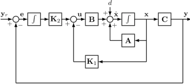
The aim is to control the position and yaw of the flying robot in the inertial coordinate axes. It is assumed that the full state is available for feedback from an on-board GPS/INS system. Hence an LQR approach is used. In order to remove steady state errors in the output, y, that are caused by distur- bances to the state derivatives, integral action is applied to the output error so that the resulting control is
u(t) =−K1x(t) +K2 Z t
0
(yr(t)−y(t))dt (23)
+ −
R K2
+ − + + +
d
B R
A
C
K1
˙ y
x x
yr e u
Fig. 5. Block diagram of system
where yr is the output reference. Assuming constant yr, differentiating (23) gives
˙
u(t) =−K1x(t)˙ −K2y(t) (24)
= [−K1A−K2C −K1B]
x(t) u(t)
(25)
= [−K1 −K2] A B
C 0 x(t) u(t)
(26) A block diagram of the system is shown in Fig 5 with an additional input disturbance vector, d(t).
To calculate the controller, the first step is to augment the system state with the control so that the augmented system input is the derivative of the control. This gives an augmented system with
Ae=
A B 0 0
, Be=
0 I
, (27)
xe= x
u
, ue= ˙u. (28)
The second stage it to use a standard LQR cost for the augmented system, that is
L= Z ∞
0
(xTeQexe+uTeReue)dt. (29) whereQeis a positive semi-definite symmetric state weighting matrix and Re is a symmetric control derivative weighting matrix. The well-known optimal state feedback controller is
Ke=R−1e BTePe (30) where Pe is the positive definite symmetric solution of the algebraic Riccati equation
ATePe+PeAe+Qe−PeBeR−1e BTePe= 0. (31) The control is thus
u˙ =−Ke
x u
(32) The final step is to equate (32) with (26) so that
Ke= [K1 K2] A B
C 0
(33) giving, provided the plant is square,
[K1 K2] =Ke
A B C 0
−1
. (34)
The final closed loop system is given by
x˙
˙ ei
=
A−BK1 BK2
−C 0 x ei
+ 0 I
I 0 yr
d y
u
=
C 0
K1 −K2
x ei
+ 0 0
0 0 yr
d
(35)
whereei(t) =Rt
0(yr(t)−y(t))dt.
IV. SIMULATION RESULTS
The flying robot that has been developed can a steady hover point despite disturbances such as wind gusts by the control system designed in this study. In this section, the control system is tested under simulation. The effect of the nonlinearities which results in interaction between control channels and limits on the magnitude of step references is investigated.
A. The controller
The control system proposed in Section III is tested with a simulation of the vehicle using the model developed in Section II. The parameters for the model are
m= 0.650kg, Jx= 7.5×10⁻³kg.m2, (36) Jy= 7.5×10⁻³kg.m2, Jz= 15.0×10⁻³kg.m2. (37) The weighting matrices are chosen as
Qe=I16×16, Re=I4×4. (38) The resulting controllers are given by
K1=
0 0 2.1402 0 0 1.7902
0 1.5735 0 0 0.7380 0
−1.5735 0 0 −0.7380 0 0
0 0 0 0 0 0
0 0 0 0 0 0
1.7691 0 0 0.1631 0 0
0 1.7691 0 0 0.1631 0
0 0 1.1732 0 0 0.1882
(39) and
K2=
0 0 1.0000 0
0 1.0000 0 0
−1.0000 0 0 0
0 0 0 1.0000
. (40) Note that the maximum gain term has a magnitude less than 2 which appears practical. The linear plant model has no cross- coupling terms between the surge/pitch, sway/roll, heave and yaw modes, hence the controllers also lack cross-coupling terms, and are essentially of a PID type for the surge, sway, heave and yaw motions, and PD type for the pitch and roll motions.
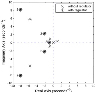
First, we examine the eigenvalues of the unregulated (open- loop) and regulated (closed-loop) system. Fig 6 shows both the open-loop and closed-loop system eigenvalues on the complex plane. All twelve of the open-loop system eigenvalues lie at the origin. The LQR regulator stabilizes the system and it can be seen that the eigenvalues lie in the left-half
−10 −8 −6 −4 −2 0 2 4 6 8 10
−10
−8
−6
−4
−2 0 2 4 6 8 10
Real Axis (seconds−1) Imaginary Axis (seconds−1 )
without regulator with regulator
12 4 2
2
2
2
Fig. 6. Eigenvalue Analysis
complex plane. Note that 4 eigenvalues lie at λ=−1.0. The remaining eigenvalues occur in complex conjugate pairs all with a damping ration of ζ = 1/√
2, which is the critical value for minimum time to peak with no oscillation. Also note that there are 2 pairs at both λ = −2.22±2.22j and λ=−8.15±8.15j.
B. Cross-coupling
The closed loop unit step responses with the linear plant are shown in Fig 7. There are no cross-coupling terms in the linear model, so these responses have not been shown.
Based on the relations (8) and (13), the non-linear model with the controller have been coded in MATLAB and the non- linear step responses obtained with ode45.m. Assuming arm lengths of0.5m, the controls are constrained to be −mg/4≤ X ≤ mg/4, −mg/4 ≤ Y ≤ mg/4, −2mg ≤ Z ≤ 0 and
−mg/24 ≤Z ≤mg/24. Anti-windup is included to set the associated controller state derivative to zero when a control constraint is active. Fig 8 shows the unit step response of the lateralxposition for the non-linear model. Although the lateral response is very close to the response for the linear system, there is a coupling to the altitude which results in a transient loss of altitude (positivez). The response to a unit demand in lateral xposition gives an identical loss in altitude, as would be expected from symmetry. The altitude and yaw responses are decoupled.
C. Reference demand limit
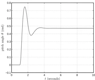
Fig 9 shows the response to a larger demand of 18m in xr. The resulting altitude loss is significant (over 40 m), but the flying robot stabilizes. The pitch response is shown in Fig 10, the pitch angle exceeds 90◦, which explains the loss in altitude. A demand of 20m results in the vehicle doing a full rotation.
0 1 2 3 4 5 6 7 8 0
0.1 0.2 0.3 0.4 0.5 0.6 0.7 0.8 0.9 1
t(seconds)
x(m)
(a)x-axis
0 1 2 3 4 5 6 7 8
0 0.1 0.2 0.3 0.4 0.5 0.6 0.7 0.8 0.9 1
t(seconds)
y(m)
(b)y-axis
0 1 2 3 4 5 6 7 8
0 0.2 0.4 0.6 0.8 1 1.2 1.4
t(seconds)
z(m)
(c) z-axis
0 1 2 3 4 5 6 7 8
0 0.1 0.2 0.3 0.4 0.5 0.6 0.7 0.8 0.9 1
t(seconds)
ψ(rad)
(d) yaw-axis Fig. 7. Closed Loop Step Responses with Linear Model
0 1 2 3 4 5 6 7 8
−0.2 0 0.2 0.4 0.6 0.8 1 1.2
lateralx,verticalz(m)
t(seconds)
lateral vertical
Fig. 8. Closed Loop Unit Step Response with Nonlinear Model
D. Simultaneous references
Fig 11 shows the flying robot response to simultaneous reference steps in all the controlled outputs. The reference step is
[xr yr zr ψr]T = [2.0 2.0 −5.0 0.1]T. (41) The responses show the vehicle tracks the target and the vehicle is stabilized.
E. Disturbance rejection
The final test is to test the ability of the robot to maintain station subject to wind disyurbances. The disturbances are modelled as for Fig 5 as disturbances to the state derivative
0 5 10 15
−10 0 10 20 30 40 50
lateralx,verticalz(m)
t(seconds)
lateral vertical
Fig. 9. Closed Loop Response to 18m Step Lateral Position Demand with Nonlinear Model
0 5 10 15
−3
−2.5
−2
−1.5
−1
−0.5 0 0.5 1 1.5
pitchangleθ(rad)
t(seconds)
Fig. 10. Pitch Angle Response to 18m Step Lateral Position Demand with Nonlinear Model
x. For example, a constant disturbance to˙ x¨ models the effect of a constant lateral wind disturbance. The response of the nonlinear model to such a disturbance
d4(t) =
0 for t <1.0
5ms−2 for t≥1.0 (42) is shown in Fig 12. The plot shows that the flying robot recov- ers and holds lateral position following the wind disturbance.
There is however a transient loss of altitude. The flying robot must hold a constant pitch of about 30◦ to counter the wind disturbance, and this is shown in Fig 13.
V. CONCLUSION
A variation of the optimal LQR has been used to design a controller for a disk-type flying robot suitable for an
0 2 4 6 8 10 0
0.2 0.4 0.6 0.8 1 1.2 1.4 1.6 1.8 2
x(m)
t
(a)x-axis
0 2 4 6 8 10
0 0.2 0.4 0.6 0.8 1 1.2 1.4 1.6 1.8 2
y(m)
t
(b)y-axis
0 2 4 6 8 10
−6
−5
−4
−3
−2
−1 0
z(m)
t
(c) z-axis
0 2 4 6 8 10
0 0.01 0.02 0.03 0.04 0.05 0.06 0.07 0.08 0.09 0.1
ψ(rad)
t
(d) yaw-axis Fig. 11. Tracking of Target
0 2 4 6 8 10
−0.1 0 0.1 0.2 0.3 0.4 0.5 0.6
lateralx,verticalz(m)
t(seconds)
lateral vertical
Fig. 12. Closed Loop Response to 5ms2 Lateral Acceleration Disturbance
observation platform for disaster countermeasures. The LQR controller is designed for the flying robot at hover. Eigenvalue analysis demonstrates the theoretical stability of the system.
The ability of the controlled robot to respond to reference demands and its disturbance rejection properties are tested by simulation of the system using a nonlinear model of the flying robot dynamics. The response for near-hover conditions is good, but for very large perturbations, the pitch and roll angles become great and this affects the ability of the controller to maintain altitude, and indeed stability. Hence for high manoeuvrability, it is envisaged that linear parameter varying [6] or nonlinear controllers [7] should be designed.
0 2 4 6 8 10
−0.1 0 0.1 0.2 0.3 0.4 0.5 0.6 0.7 0.8
pitchangleθ(rad)
t(seconds)
Fig. 13. Pitch Angle Response to 5ms2Lateral Acceleration Disturbance
Large step demands drive the robot to instability, this can be countered by shaping the reference demands to restrict the maximum demand rates. Note that the control design does not consider the actuator dynamics. In fact the control is actually generic, hence any implementation requires a controller allo- cation block, see [8] for details. In the future, the controller will be implemented and tested on the flying robot platform.
REFERENCES
[1] R. Mahony, V. Kumar, and P. Corke, “Multirotor aerial vehicles:
Modeling, estimation, and control of quadrotor,” Robotics Automation Magazine, IEEE, vol. 19, no. 3, pp. 20–32, Sept 2012.
[2] I. Yamamoto, N. Inagawa, T. Tsuji, and T. Otawa, “Research and development of the multifunctional observation and data transfer system for disaster prevention,” inProceedings of the 4th International Congress on Image and Signal Processing (CISP 2011), Shanghai, China, Oct.
2011.
[3] T. Matsuzaki, I. Yamamoto, N. Inagawa, T. Nakamura, W. Batty, and J. F. Whidborne, “Development of unmanned flying observation robot with real time video transmission system,” in Proc. World Automation Congress (WAC 2010), Kobe, Japan, Sep. 2010, p. 5 pages, article number 5665710. [Online]. Available: http://wacong.org/Finalprogram.html [4] L. Derafa, A. Benallegue, and L. Fridman, “Super
twisting control algorithm for the attitude tracking of a four rotors UAV,” Journal of the Franklin Institute, vol. 349, no. 2, pp. 685–699, 2012. [Online]. Available:
http://www.sciencedirect.com/science/article/pii/S0016003211002821 [5] N. Inagawa, I. Yamamoto, and T. Nakamura, “Application of unmanned
flying observation robot using real time video transmit system,”Journal of Electrical Engineering Theory and Application, vol. 12010, no. Iss.
2, pp. 86–91, 2010.
[6] S. L. M. D. Rangajeeva and J. F. Whidborne, “Linear parameter varying control of a quadrotor,” in 6th IEEE International Conference on Industrial and Information Systems (ICIIS), Kandy, Sri Lanka, Aug.
2011, pp. 483–488. [Online]. Available: http://www.iciis2011.org/
[7] A. Marks, “A fault hiding approach for fault tolerant control of a novel VTOL vehicle,” Ph.D. dissertation, Cranfield University, Bedfordshire, UK, 2014.
[8] A. Marks, J. F. Whidborne, and I. Yamamoto, “Control allocation for fault tolerant control of a VTOL octorotor,” in UKACC International Conference on Control 2012, Cardiff, U.K., Sep. 2012, pp. 357 – 362.