ファジィ微分方程式の解の吸引性について (関数方程式の定性的理論とその現象解析への応用)

ファジィ微分方程式の解の吸引性について

大阪大学大学院工学研究科応用物理学専攻 齋藤誠慈(Seiji Saito)

GraduateSchoolof Engineering, Osaka University

E-mail:[email protected]

Keywords : FuzzyNumbers;FuzzyDifferential Equations; Attractivity Set; Couple Parametric

Representation;

1Introduction

There are many fruitful results on the

representations of fuzzy numbers, differentials

and integrals of fuzzy functions (see, e.g.,

in Goetschel-Voxman $[8, 9]$, Dubois-Prade [3,

4, 5, 6], Puri-Ralescue [13], Furukawa [7],

Kaleva $[10, 11]$ etc). They establish

funda-mental results concerning differentials, inte

grals and fuzzy differential equations of fuzzy

functionswhichmap $\mathrm{R}$to aset of fuzzy

num-bers. By usingthe results it seems to be

dif-ficultto aPPlyall the practical and significant

problems. In this studying we introduce the

couple parametric representation [2]$)$

cor-responding tothe representationof fuzzy

num-bers due toGoetschel-Voxmansothatitiseasy

to solve fuzzy differentialequations.

In Buckley [1], Kaleva$[10, 11]$, Park [12] and

Song [16], various types of conditions for the

existence and uniqueness ofsolutions to fuzzy

differentialequations. By thecouple

represen-tation some kinds of differential and integral

of fuzzy functions can be easily treated in an

analogous waywith thereal analysisaswellas

some tyPe of fuzzy differential equations

can

be solved without difficulty.

In Section 2we denote afuzzy number $x$

by$(a, b)$, where$a,b$areendpointsof at-cut set

of the membership function $\mu_{x}$

.

Wegive some

kind of metric spacewhich includes the set of

fuzzy numbers as well as prove the continuity

of$a$,$b$

.

In Section3we give definitions of

differ-entialandintegral of fuzzy functionsand

suffi-cient conditions for fuzzy functions to be

differ-entiableorintegrable. InSection4wegetbasic

results of existence and uniqueness ofsolutions

for fuzzydifferentialequations byaPPlying the

contraction principle. In Section 5we treat

afuzzy differential equation $x’=p(t)x,\mathrm{w}\mathrm{h}\mathrm{e}\mathrm{r}\mathrm{e}$

$p(t)$ is afuzzy valued function, and we

calcu-late the the exponential function $e^{x}$, where $x$

is afuzzy number. In the section weshow the

attractivityset,where all thesolutionsare

aP-proaching to the zero as the time increasing

the infinity

数理解析研究所講究録 1216 巻 2001 年 255-265

2Parametric

Representa-

We introduce the following parametric

reP-tion

of Fuzzy Numbers

resentationof$\mu\in F_{\mathrm{b}}^{st}$,

Inorder to introduceametric spacewhich

includes the set of fuzzy numbers,

we

define

the following set.

$a(\alpha)$ $=$ $\min L_{\alpha}(\mu)$,

$b(\alpha)$ $=$ $\max L_{\alpha}(\mu)$

$.11\cdot \mathrm{w}111\epsilon$$\infty\cup\cdot$

for$0<\alpha\leq 1$ and

$X=\{x=(a, b)\in C(I)\mathrm{x}C(I)\}$

$r$ ’ $\backslash$

where $I=[0,1]$and$C(I)$ isthe setof

continu-ous

functions from I to R. Denote ametric by

$d(x,y)= \sup_{\alpha\in I}(|a(\alpha)-c(\alpha)|+|b(\alpha)-d(\alpha)|)$

for$x=(a,b),y=(c,d)\in X$

.

Then the metric

space $(X,d)$ is complete.

Definition 1Consider

a

set fuzzy numbers

with bounded supports

as

_follows:

$F_{\mathrm{b}}^{\iota t}=$

{

$\mu:\mathrm{R}arrow I$ satisfying $(i)-(iv)$

below.}

(i) There exist

a

unique $m\in \mathrm{R}$ such that

$\mu(m)=1$;

(ii) The set sum(\mu )=d({\mbox{\boldmath $\xi$}\in R: $\mu(\xi)>0\}$)

is bounded in$\mathrm{R}$;

(iii) One

_of

the following conditionsholds;

(a)$\mu$ is strictly$f.i$fuzzy convex, $i.e.$,

$\mu(c\xi_{1}+(1-c)\xi_{2})>\mathrm{m}$$\dot{\mathrm{m}}[\mu(\xi_{1}),\mu(\xi_{2})]$

for

$\xi_{1},\xi_{2}\in \mathrm{R}$, $0<c<1$;

(b)$\mu(m)=1$ and$\mu(\xi)=0$

for

$\xi\neq m$;

(iv) $\mu$ is uppersemi-continuous

on

R.

Remark 1The above condition (iiia) is

stronger than

one

inthe usual

case.

It

_follows

that$\mu(\xi)$ is strictly increasing in$( \in(-\infty,m)$

and strictly decreasing in $\xi\in(m, \infty)$

.

This

condition plays

an

importantrole in $\theta\iota e$ proof

of

Theorem 1.

$L_{\alpha}(\mu)$ $=$ $\{\xi\in \mathrm{R}:\mu(\xi)\geq\alpha\}$,

$a(0)$ $=$ $\min cl(sfu_{fl}(\mu))$,

$b(0)$ $=$ $\max d(suw(\mu))$

.

SeeFigure 1.

Remark 2 fi}$\eta m$ the extension principle

of

Zadeh, it

_follows

that

$\mu_{x+y}(\xi)$

$=\epsilon^{\max_{=}\min_{\xi_{1}+\xi_{2}\cdot=1,2}(\mu:(\xi)))}.$

:

$= \max\{\alpha\in I:\xi=\xi_{1}+\xi_{2},\xi:\in L_{\alpha}(\mu_{i})\}$

$= \max\{\alpha\in I:\xi\in[a(\alpha)+c(\alpha),b(\alpha)+d(\alpha)]\}$,

where $\mu_{1}$,$\mu 2$

are

membership

functions of

$x$,$y$,

respectively. Thus

we

get$x+y=(a+c, b+d)$

.

The following theorem is abasic result.

Theorem 1Denote $\mu=(a,b)\in F_{\mathrm{b}}^{st}$, where

$a,b$ : $Iarrow \mathrm{R}$

.

The followingprvperties(i)-(iii)

hold:

(i) a,b

are

continuous

on

Ij

(ii) $\max a(\alpha)=a(1)=m$ and $\min b(\alpha)=$

$b(1)=m_{j}$

(iii)

One

_of

the

_follow

$.ng$statements holds;

(a)$a$ is strictly increasingand$b$is strictly

decreasing with$a(\alpha)<b(\alpha)$;

(b)$a(\alpha)=b(\alpha)=m$

for

$0<\alpha<1$

.

Conversely, under the above conditions (i)

$-(iii)$,

if

we denote

$\mu(\xi)=\sup\{\alpha\in I$:$a(\alpha)\leq\xi\leq b(\alpha)\}$

then$\mu\in F_{\mathrm{b}}^{st}$

.

Moreoverit

follows

thatR$\subset F_{\mathrm{b}}^{st}$

and that$F_{\mathrm{b}}^{st}$ is a closed convex cone inX.

In the following examplewe illustrate

tyPi-cal three typesof fuzzy numbers.

Example 1Consider the following $L-R$

fuzzynumber$x\in F_{\mathrm{b}}^{st}$ withamembership

func-tion as

_follows:

$\mu_{x}(\xi)=\{$

$L( \frac{m-\xi}{\iota})_{+}$

for

_{$\xi\leq m$} $R( \frac{\xi-m}{r})_{+}$

for

$\xi>m$

where$m\in \mathrm{R}$,$l>0$,$r>0$

.

$L$,$R$ are into

maP-pings

_defined

on $\mathrm{R}^{+}=[0, \infty)$

.

Let $L(\xi)_{+}=$

$\max(L(\xi), 0)$ etc. We identify $\mu_{x}$ with $x=$

$(a, b)$ Then we have $a(\alpha)=m-L^{-1}(\alpha)l$ and

$b(\alpha)=m+R^{-1}(\alpha)r$ provided that $L^{-1}$ and

$R^{-1}$ eist.

Let $L(\xi)=-c_{1}\xi+1$, where $c_{1}>0$

.

We

illustrate the following cases $(a)-(c)$

.

(i) Let $R(\xi)=-\mathrm{c}2\mathrm{f}+1$, where $c_{2}>0$

.

Then

$c_{2}l(b-m)=c_{1}r(m-a)$

.

(ii) Let$R(\xi)=-c_{2}\sqrt{\xi}+1$, where$c_{2}>0$

.

Then

$c_{2}l(b-m)^{2}=c_{1}r^{2}(m-a)$

.

(ii) Let$R(\xi)=-c_{2}\xi^{2}+1$, where$c_{2}>0$

.

Then $c_{2}^{2}l^{2}(b-m)=c_{1}^{2}r(a-m)^{2}$

.

See Figure 2.

3Differential

and Integral

of

Fuzzy

Valued

Func-tions

Let

an

interval $J\subset \mathrm{R}$

.

We callafunction

$x$ : $Jarrow F_{\mathrm{b}}^{st}$ to be afuzzy valued function.

Denote

$x(t)$ $=$ $(a(t),b(t))$

$=$ $\{(a(t, \alpha), b(t, \alpha))^{T}\in \mathrm{R}^{2}$:$\alpha\in I\}$

.

We definethe continuietyand

differentiabil-ityof fuzzy valued function asfollows:

Definition 2A fuzzy valued

_function

$x$ : $Jarrow$

$F_{\mathrm{b}}^{st}$ is continuous at$t\in J$

if

$\lim_{harrow 0}d(x(t+h), x(t))=0$

.

Denote the set

_of

all the continuous

_functions

$x:Jarrow F_{\mathrm{b}}^{st}$ by$C(J)$

.

Let the

_function

$x:Jarrow F_{\mathrm{b}}^{st}$ by

$x(t)$ $=$ $\{(a(t, \alpha), b(t, \alpha))^{T}\in \mathrm{R}^{2} : \alpha\in I\}$

$=$ $(a(t, \cdot), b(t, \cdot))=x(t$,$\cdot$$)$

for

$t$ $\in$ J. The

function

$x$ is

dif-ferentiable

at $t$ $\in$ $J$

if for

any $\alpha$ $\in$

I there eist $\frac{\partial a}{\partial t}(t, \alpha)$,$\frac{\partial b}{\partial t}(t,\alpha)$ such that $\frac{\partial a}{\partial t}(t, \alpha)\leq\frac{\partial b}{\partial t}(t, \alpha)$ and $\mu(t, \cdot)\in F_{\mathrm{b}}^{st}$, where

$\mu(t,\xi)=\sup\{\alpha\in I$ : $\frac{\partial a}{\partial t}(t, \alpha)$ _$\leq\xi$ $\leq$ $\frac{\partial b}{\partial t}(t, \alpha)\}$

.

The

function

$x$ is

differentiable

on

$J$

if

$x$ is

differentiable

at any $t\in$ J.

De-note $\frac{dx}{dt}(t)=x^{l}(t)=(\frac{\partial a}{\partial t}(t, \cdot), \frac{\partial b}{\partial t}(t, \cdot))$ and it

is called to be the derivative

_of

$x(t)$

.

We define an integral of an $F_{\mathrm{b}}^{st}-$ valued

function x.

Definition 3Let x : J $arrow \mathcal{F}_{\mathrm{b}}^{\epsilon t}$ be $x(t, \cdot)=$ ball by B $=$

{x

$\in F_{\mathrm{b}}^{st}$:$d(x, 0)\leq 1\}$

.

Define

$(a(t,$.),$b(t, \cdot))$

for

t $\in$ J. The

function

x is rB $=$

{rx

$\in F_{\mathrm{b}}^{st}$: x$\in B\}$ for r $>0$

.

called to be integrable over $[t_{1}, t2]$, since $a$,$b$ Assumption (A) Let$r>0$ and

ore

Riemann integrable

over

$[t_{1}, t_{2}]$

.

Then we

$B(x_{0}, r)=x0+rB$

.

define

the integralas

_follows:

The following conditions (i) and (ii) are

satis-$\int_{t_{1}}^{t_{2}}x(s, \cdot)ds$

fied.

$=$ $\{(\int_{t_{1}}^{t_{2}}a(s, \alpha)ds, \int_{t_{1}}^{t_{2}}b(s, \alpha)ds)^{T}\in \mathrm{R}^{2} : \alpha\in I\}.(\mathrm{i})$ It follows that $f(t, x)$ $\in$

$F_{\mathrm{b}}^{st}$ for any

$(t, x)\in J_{\mathrm{c}}\mathrm{x}B(x_{0}, r)$, i.e., for any _$x=$

Remark 3Let $x(t)=(a(t,$.),$b(t, \cdot))$ $\in F_{\mathrm{b}}^{st}$

$\{(a(\alpha), b(\alpha)) : \alpha\in I\}\in F_{\mathrm{b}}^{st}$,$t\in J_{c}$ the

for

$t\in J$

.

following properties$(\mathrm{a})-(\mathrm{c})$ hold for$t\in J$:

(%)

_If

$x$ is

differentiate

at$t$,

we

get the

inte-gralover $[t_{1}, t2]\subset J$

as

follows:

$\int_{t_{1}}^{t_{2}}x(s, \cdot)ds=x(t2, \cdot)-x(t1’, \cdot)$

.

(ii)

_If

$x(t)\in F_{\mathrm{b}}^{st}$ is integrable

over

$[t_{1},t_{2}]$,

then

we

have$\int_{t_{1}}^{t_{2}}x(s, \cdot)ds\in F_{\mathrm{b}}^{\epsilon t}$

.

And also

we

have

$d( \int_{t_{1}}^{t_{2}}x(s, \cdot)ds,0)\leq\int_{t_{1}}^{t_{2}}d(x(s, \cdot), a)ds$,

4Fuzzy

Differential

Equa-tion I

Consider

an

initial value problem of

adif-ferential equation in the metric space$X$

as

fol-lows:

$x(t)=f(t,x)’$, $x(t\mathrm{o})=x0$ (N)

where $t0\in \mathrm{R},x0\in F_{\mathrm{b}}^{\epsilon t}$

.

Let $f$ : $J_{c}\cross Xarrow X$,

where $J_{\mathrm{c}}=[t_{0},t0+c],c>0$

.

We call the

equationof(N)tobe afuzzydifferentialequa

tion if $f(t, x)$ is afuzzyvalued function

on a

subset of $J_{\mathrm{c}}\mathrm{x}X$

.

Moreover

we

assume

that

the following assumption. Denote the unit

(a) $f_{\dot{1}}(t, (a(\alpha),b(\alpha)),$$\alpha)$,$i$ $=$ 1, 2, are

contiunous in $\alpha$;

(b) For each $t\in J$ there exists aunique

value $M(t)\in \mathrm{R}$such that

$\max_{\alpha}f_{1}(t, (a(\alpha), b(\alpha)),$$\alpha)$

$=f1(t, (a(1), b(1))$,$1)=M(t)$;

$\min_{\alpha}f_{2}(t, (a(\alpha), b(\alpha)),$ $\alpha)$

$=f_{2}(t, (a(1), b(1))$,$1)=M(t)$;

(c) One of the following statements

holds;

(a) $f_{1}(t, (a(\alpha),b(\alpha)),\alpha)$ is

strictly increasing in at and

$f_{2}(t, (a(\alpha), b(\alpha))$,$\alpha)$ is strictly

decreasingin $\alpha$;

(b) $f_{1}(t, (a(\alpha), b(\alpha))$,ci) $=$

$f_{2}(t, (a(\alpha), b(\alpha))$,$\alpha)$ for$0<\alpha<1$

.

(ii) Function $f(t,x)$ is continuous on $(t,x)\in$

$J_{\mathrm{c}}\mathrm{x}B(x_{0},r)$

.

In the

same

way in the theory ofordinary

differential equations

we

give the following

def-initionof solutions for initial value problems of

fuzzy differentialequation

Definition 4Let $J_{1}$ be an intemal in R and Example 2Considerthe

follow

ing problem

of

$t_{0}\in J_{1}$. A

function

$x$ : $J_{1}arrow F_{\mathrm{b}}^{st}$ is a

solu-tion

_of

(N) on $J_{1},ifx$

satisfies

the following

conditions $(i)-(iii)$

.

(i) $x(t_{0})=x_{0;}$

(ii) $x(t)\in F_{\mathrm{b}}^{st}$

for

$t\in J_{1}$;

(Hi) There exists $x’(t)$ _and $x^{t}(t)=f(t, x(t))$

for

$t\in J_{1}$.

By aPPlying the contraction principleweget

the following theorem.

Theorem 2Suppose that the following

condi-tions (i) and (ii) are

_satisfied

under

Assump-tion (A) :

(i) $f$ is bounded, $i.e.$, there eists an $M>0$

such that

$d(f(t, x),0)\leq M$

for

$(t, x)\in J_{c}\mathrm{x}B(x_{0}, r)$;

(ii) $f$ is Lipschitzian in$x,i.e.$, there eists an

$L>0$ such that

$d(f(t,x)$,$f(t, y))\leq Ld(x,y)$

for

$(t, x)$,$(t, y)\in J_{c}\mathrm{x}B(x_{0}, r)$

.

Then there eists a unique solution$x$

for

(N)

such that

$x(t)=x_{0}+ \int_{t_{\mathrm{O}}}^{t}f(s, x(s, \cdot))ds$

$for$$t\in J_{\rho}=[t_{0},t_{0}+\rho]$, where$\rho=\min(c, r/M)$

.

We illustrate theabovetheoremby aPPlying

it to the following example.

fuzzy

_differential

equation

$x^{l}=p(t)x+q(t)$_, $x(t_{0})=x0$ (E)

$t\in \mathrm{R}$,$x_{0},x(t)\in F_{\mathrm{b}}^{st}$

.

Functions_$p,q$ : $\mathrm{R}arrow \mathrm{R}$

are continuous.

Let$f(t, x)=p(t)x+q(t)$and$p(t)\geq 0$

.

Since

$d(f(t, x)$,0) $\leq$ $p(t)d(x, \mathrm{O})+|q(t)|$,

$f(t, x)$ $\in$ $f(t,y)+p(t)d(x, y)B$,

itfollowsthat$f$isboundedand Lipschitzian in

$x$

.

Prom Theorem 2we haveauniquesolution

of (E) suchthat

$x(t)=e^{\int_{\iota_{\mathrm{O}}}^{t}p(s)ds}x_{0}+ \int_{t_{\mathrm{O}}}^{t}e^{\int_{l}^{t}p(r)dr}q(s)ds$

for$t\in \mathrm{R}$

.

Let $p$ : $\mathrm{R}$ $arrow$ $(-\infty,0]$ and

$x(t)$ $=$ $(x_{1}(t), x_{2}(t))$

.

Then we have

$x_{1}(t)’=p(t)x_{2}(t)+q(t)$,$x_{2}^{J}=p(t)x_{1}(t)+q(t)$,

by denoting $x0=(a0, b_{0})$, so $x_{1}(t, \alpha)$ and

$x_{2}(t, \alpha)$ satisfy

$(\begin{array}{l}x_{1}(t,\alpha)x_{2}(t,\alpha)\end{array})=\Phi(t, \alpha)$ $(\begin{array}{l}a_{0}(t,\alpha)b_{0}(t,\alpha)\end{array})$

$+ \Phi(t, \alpha)\int_{t_{\mathrm{O}}}^{t}\Phi^{-1}(s, \alpha)$ $(\begin{array}{ll}q(s \alpha)q(s,\alpha) \end{array})$ $ds$,

where $\Phi(\cdot$,$\cdot$$)$ isafundamental matrix of

$\frac{d}{dt}(x_{1}(t, \alpha),$$x_{2}(t, \alpha))^{T}$

$=(p(t, \alpha)x_{2}(t, \alpha),p(t, \alpha)x_{1}(t, \alpha))^{T}$

$,\mathrm{i}.\mathrm{e}.$,

$\Phi(t, \alpha)$ $=$ $(\begin{array}{ll}\phi_{11}(t,\alpha) \phi_{12}(t,\alpha)\phi_{21}(t,\alpha) \phi_{22}(t,\alpha)\end{array})$

$e^{\int_{t_{\mathrm{O}}}^{t}p(s,\alpha)ds}+e^{-\int i_{0}^{p(s,\alpha)ds}}$ $\phi_{11}(t, \alpha)$ $=$

2

$e \mathrm{o}-e\int_{t}^{t}p(s,\alpha)ds-\int_{\iota_{0}}^{t}p(s,\alpha)ds$ $\phi_{12}(t,\alpha)$ $=$ 2 $e^{\int_{t}^{t}p(\epsilon,\alpha)d\epsilon}\mathrm{o}-e^{-\int_{c_{0}}^{t}p(s,\alpha)ds}$ $\phi_{21}(t,\alpha)$ $=$ 2 $e \mathrm{o}+e\int_{t}^{t}p(s,\alpha)d\epsilon-\int_{\iota_{0}}^{t}p(s,\alpha)ds$ $\phi_{22}(t,\alpha)$ $=$ 2 for t $\geq t_{0},\alpha\in I$

.

5Fuzzy

Differential

Equa-$\mathrm{t}\mathrm{i}\dot{\mathrm{o}}\mathrm{n}$

II

We considerthe exponentialfunction$e^{x}=$

$\sum_{\dot{|}=0}^{\infty}\frac{xx^{l}}{\vec{|}\Gamma}$, where _{$x\in Fi^{t}$}, inthe similar to the

real analysis.

Let $x=(a, b)$, then $\alpha$-cut sets of

mem-bership function $\mu_{x}$ is $L_{\alpha}(\mu_{x})=[a(\alpha),b(\alpha)]$

for $\alpha\in I$

.

We calculate $x^{:},i=2,3$,$\cdots$, in

the following

cases

$(a)-(c)$

.

By the extension

principleofZadeh, it follows that

$\mu_{x}$‘$(\xi)$

$=$ $\max$ $\min(\mu(\xi_{\mathrm{j}}))$

$\epsilon=\mathrm{n}_{f}\epsilon_{J}1\leq \mathrm{j}\leq$

:

$=$ $\max\{\alpha\in I: \langle =\Pi_{j}\xi_{j},\xi_{j}\in L_{\alpha}(\mu_{x})\}$

.

When i $=2$,

we

find the followingrelations,

(a) If$0\leq a(\alpha)\leq b(\alpha)$,then

we

get

$L_{\alpha}(\mu_{xx^{2}})=[a(\alpha)^{2},b(\alpha)^{2}]$,

Thus$x^{2}=(a^{2},b^{2})\in F_{\mathrm{b}}^{\iota t}$

.

(b) If$a(\alpha)\leq b(\alpha)\leq 0$,then

we

have

$L_{\alpha}(\mu_{x}\mathrm{a})=[b(\alpha)^{2},a(\alpha)^{2}]$,

th$\mathrm{u}\epsilon$ $x^{2}=(b^{2},a^{2})\in F_{\mathrm{b}}^{\iota t}$

.

(c) If$a(\alpha)\leq 0\leq b(\alpha)$, thenitfollows that

$L_{\alpha}(\mu_{x^{2}})=[a(\alpha)b(\alpha), c(\alpha)]$

where $c( \alpha)=\max(a(\alpha)^{2}, b(\alpha)^{2})$

.

With-out loss of generalitywe denote$\mu_{x}$ bythe

membership function in Examplel. De

note

$L^{-1}(\alpha+h)$ $=$ $L^{-1}(\alpha)+\Delta_{1}$,

$R^{-1}(\alpha+h)$ $=$ $R^{-1}(\alpha)+\Delta_{2}$,

where $\Delta_{1}<0$,$\Delta_{2}<0$ for $h>0$

.

Then we

have $a(\alpha+h)b(\alpha+h)-a(\alpha)b(\alpha)$ $=$ $a(\alpha)\Delta_{2}r-b(\alpha)\Delta_{1}l-\Delta_{1}\Delta_{2}lr>0$. Since $a(\alpha+h)$ $=$ $a(\alpha)-\Delta_{1}l<0$, $b(\alpha+h)$ $=$ $b(\alpha)-\Delta_{2}r>0$, then

we

have $(a(\alpha)-\Delta_{1}l)\Delta_{2}r>0$, $(b(\alpha)-\Delta_{2}r)\Delta_{1}l<0$

.

Thus ab is increasing in$\alpha$and in thesame

way $c$ is decreasing. And $x^{2}=$ (ab, c) $\in$

$F_{\mathrm{b}}^{\epsilon t}$

.

From the above discussion

we

give the

fol-lowing definition.

Definition

_5Define

$e^{x}= \sum_{\dot{|}=0}^{\infty}\frac{x^{\dot{l}}}{\dot{\iota}!}\in F_{\mathrm{b}}^{\epsilon t}$

for

x$\in F_{\mathrm{b}}^{\iota t}$

.

The followingtheorem shows the

represen-tation of$e^{x}$ for

x

$\in F_{\mathrm{b}}^{\epsilon t}$

.

Theorem 3Let$x=(a, b)\in F_{\mathrm{b}}^{\epsilon t}$

.

Thenweget

thefollowing representation

_of

the fuzzy

num-bet$e^{x}$

as

follows:

(i)

_If

$0\leq a(\alpha)\leq b(\alpha)$, then we have (i) Let$p_{1}(t, \alpha)\geq 0$ on $\mathrm{R}\cross I$ and an initial

$e^{x}=(e^{a}, e^{b})$

$=\{(e^{a(\alpha)}, e^{b(\alpha)})^{T}\in \mathrm{R}^{2} : \alpha\in I\}$

.

(ii)

_If

$a(\alpha)\leq b(\alpha)\leq 0$, then we get

$e^{x}= \frac{e^{a}+e^{b}}{2}+(-\frac{e^{-a}-e^{-b}}{2}, \frac{e^{-a}-e^{-b}}{2})$

.

In somecasethe following property holds.

condition$x_{0}=(a0, \mathrm{b})$

.

Then the solution

$x=(x_{1},x_{2})$

of

$(E_{0})$ is described by

$x(t,\alpha)=(e^{\int_{\tau}^{\mathrm{t}}p_{1}(s,\alpha)d\epsilon}a(\alpha), e^{\int_{\tau}^{t}\mathrm{P}2(s,\alpha)d\epsilon}b(\alpha))$

as long as $x_{1}$($t$,ce) $\geq 0$

for

$t\in J_{1},\alpha\in$

$I$, where $J_{1}$ is an interval in $[\tau, \infty)$ and

$x(\tau)=(a(\alpha), b(\alpha))$

.

It

follows

that

Theorem 4Let $x=(a,b)\in F_{\mathrm{b}}^{st}$ and _$y=$

$(c, d)\in F_{\mathrm{b}}^{st}$ with $a(\alpha)\geq 0$ and$c(\alpha)\geq 0$

for

$at\in I$

.

then we have

$x(t,\alpha)=(e^{\int_{\tau}^{t}p_{2}(s,\alpha)ds}a(\alpha), e^{\int_{\tau}^{t}p_{2}(s,\alpha)ds}b(\alpha))$

as longas$x_{1}(t, \alpha)\leq 0\leq x_{2}(t, \alpha)$ and that

$e^{x}e^{y}=e^{x+y}$

.

$x(t, \alpha)=(e^{\int_{\tau}^{t}p_{2}(\epsilon,\alpha)ds}a(\alpha), e^{\int_{\tau}^{t}p_{1}(s,\alpha)ds}b(\alpha))$

Example 3Consider behaviors

_of

solutions

of

the following problem

_of

afuzzy

_differential

equation

$x=p(t)x$, $x(t_{0})=x0$ _(Eo)

where $t\in \mathrm{R}$,$x_{0}$ and $x(t)\in F_{\mathrm{b}}^{st}$

.

Function

$p(t)=(p_{1} (t, \cdot),p_{2}(t, \cdot))$ : $\mathrm{R}arrow F_{\mathrm{b}}^{st}$ is

contin-uous.

Remark4Let $T(x)=p(t)x$

.

It

_follows

that

$T$ is non-linear.

In analyzing the ordinary differential

equa-tion $x$

’

$=$ $a(t)x+\mathrm{b}(\mathrm{a})$, where $a$,$b$ : $\mathrm{R}arrow \mathrm{R}$ are continuous, the condition that

$\lim_{tarrow\infty}\int^{t}a(s)ds=0$plays an important role in

showingthe propertythat $\lim_{tarrow\infty}x(t)=0$

.

Conserning fuzzy differetial equation $(E_{0})$, we

getanextensionresultofasymptoticbehaviors

of ordinary lineardifferentialequations aswell

as weobservealittledifferent resultasfollows.

Theorem 5Consider Problem $(E_{0})$

.

The

fol-louting cases (i) and (ii) hold:

as long as $x_{2}(t, \alpha)\leq 0$

for

t$\in J_{1},\alpha\in I$

.

(ii) Let $p_{2}(t, \alpha)\leq 0$ on $\mathrm{R}\mathrm{x}$ I. As long as

$x_{1}(t, \alpha)\geq 0$ or$x_{2}(t, \alpha)\leq 0$

for

$t\geq\tau$,$\alpha\in$

$I$, it

follows

that

$d(x(\tau, \cdot)$,$0)e^{\int_{\tau}^{t}p_{1}(s,\cdot)ds}$

$\leq d(x(t, \cdot),$ $0)$

$\leq d(x(\tau, \cdot),0)e^{\int_{\tau}^{t}p_{2}(s,\cdot)ds}$

where $\tau\geq t_{0},t\geq\tau,\alpha\in I$

.

As long as

$x_{1}(t, \alpha)\leq 0\leq x_{2}(t, \alpha)$

for

$t\geq\tau$,a $\in I$, it

follows

that

$d(x(\tau, \cdot)$_,$0)e^{-\int_{\tau}^{t}p_{2}(\epsilon,\cdot)ds}$

$\leq d(x(t, \cdot),$$0)$

$\leq d(x(\tau, \cdot)$,$0)e^{-\int_{\tau}^{t}p_{1}(*,\cdot)ds}$

$t\geq\tau$,$\alpha\in I$

.

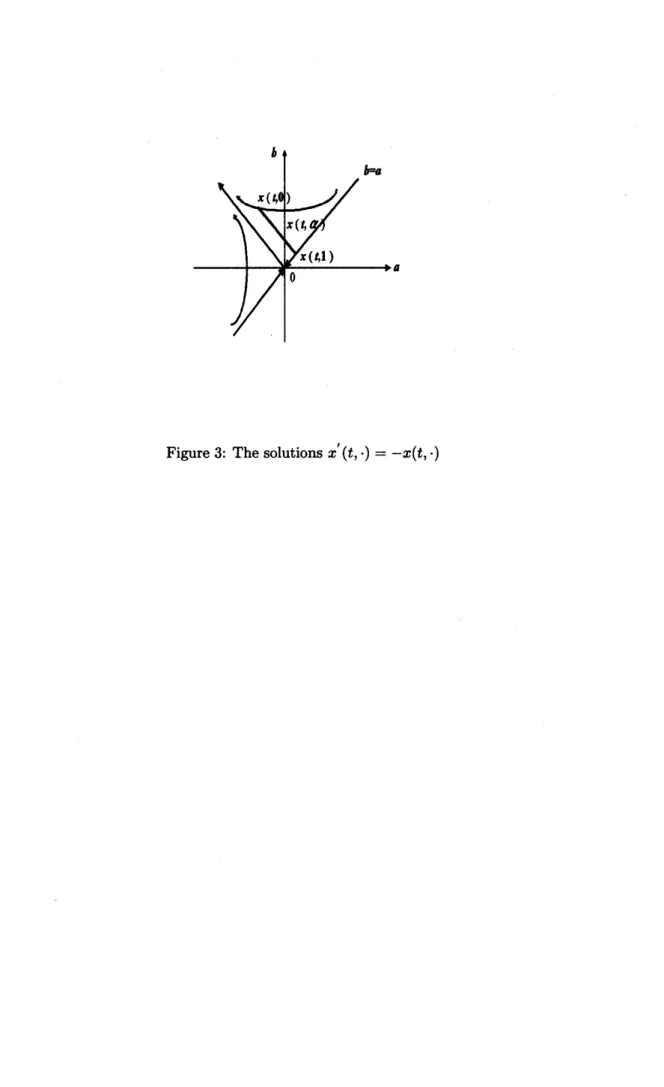
Example 4Consider Problem $(E_{0})$ with

$x(t_{0})$ $=$ $(a_{0},b_{0})$ $\in$ $F_{\mathrm{b}}^{st}$

.

Suppose that

$\lim_{tarrow\infty}\int_{t\mathrm{o}}^{t}p_{2}(t, \alpha)=-\infty$

for

$t_{0}\in \mathrm{R}$,$\alpha\in I$

.

Seikkala [15] calculates the solution in case

that $p(t)\equiv-1$

.

SeeFigure3.

In the following theorem

we

showan

attrac-tivity set $A^{E_{0}}(t_{0})$ of$(E_{0})$ at

to

$\cdot$ Here

$A^{E_{0}}(t_{0})$

is asubset of$F_{\mathrm{b}}^{st}$ as follows:

Definition

_6If

$x0\in A^{E_{0}}$(to), then all the

s0-lutions$x$

of

$(E_{0})$passingthrough$(t_{0}, x_{0})\in \mathrm{R}\mathrm{x}$

$F_{\mathrm{b}}^{\epsilon t}$

satisfies

$\lim_{tarrow\infty}d$($x$($t$,ci),$0$) $=0$

for

$at\in I$

.

It is clear that $x_{0}=0\in A^{E_{0}}(t_{0})$ for any

$t0\in \mathrm{R}$

.

In the

case

that$p_{1}(t, \alpha)\equiv \mathrm{p}\mathrm{i}(\mathrm{t},\mathrm{a})\leq 0$

and $t \lim_{arrow\infty}\int_{\iota_{\mathrm{o}}}^{t}p_{1}(s,\alpha)ds=-\infty$ for $t_{0}\in \mathrm{R},\alpha\in$

$I$, it followsthat $A^{E_{0}}(t_{0})=\mathrm{R}$ for$t_{0}\in \mathrm{R}$

.

When $p_{1}(t, \alpha)$

I

$p_{2}(t, \alpha)$,

we

have the

fol-lowing theorem.

Theorem 6Consider Problem $(E_{0})$ with

$p_{1}(t)$

I

$P2(t)$

.

Let$p_{2}(t,\alpha)\leq 0$

on

$\mathrm{R}\mathrm{x}$ I and

$\lim_{tarrow\infty}\int_{t_{0}}^{t}p_{2}(s, \cdot)ds=-\infty$

for

$t\mathit{0}\in \mathrm{R}$

.

Then

we

have$A\ (t_{0})=\{\mathrm{O}\in \mathrm{R}\}$

for

any$t_{0}\in \mathrm{R}$

.

Theabove theorem isprovedin [14]. Consider

the following problem

$x=P_{m}(t)x’$, $x(t\mathrm{o})=x0$ $(P_{m})$

$P_{m}$ : $\mathrm{R}arrow F_{\mathrm{b}}^{\epsilon t}$suchthat$P_{m}=(-m-q_{1},$$-m+$

$q_{2})$satisfying

$m:\mathrm{R}\mathrm{x}Iarrow \mathrm{R}$,$m(t, \alpha)\geq 0$,

q: : RxI$arrow \mathrm{R}$,

where $q(t, \alpha)=\max(q_{1}(t, \alpha),$$q_{2}(t, \alpha))$

.

Then

for

any solution x $=(x_{1},x_{2})$

of

$(P_{m})$ it

fol-lows that

$\lim_{tarrow\infty}|x_{1}(t, \alpha)+\mathrm{P}2(\mathrm{t}, \alpha)|=0$

for

$\alpha\in I$

.

References

[1] J. Buckley, T. Feuring, Fuzzy Differential

Equations, Fuzzy Sets and Systems 110

(2000) , 4354.

[2] M. Chen,S. Saito, H. Ishii,Representation

of Fuzzy Numbers and Fuzzy Differential

Equations (to be submitted to Fuzzy Sets

and Systems).

[3] D. Dubois, H. Prade, Operationson Fuzzy

Numbers, Internat. J. of Systems9(1978),

613626.

[4] D. Dubois, H. Prade, Towards Fuzzy

Dif-ferential Calculus Part I:Integration of

Fuzzy Mappings, Fuzzy Sets and Systems

8(1982), 1-17

[5] D. Dubois, H. Prade, Towards Fuzzy

Dif-ferential Calculus Part II :Integration of

Fuzzy Intervals, FuzzySets and Systems 8

(1982), 105-116.

$0\leq q*\cdot(t, \alpha)\leq m(t, \alpha),$i$=1,$2. [6] D. Dubois, H. _{Prade, Towards Fuzzy}

Dif-Theorem 7Suppose that

_for

$\alpha\in I$,$t0\in \mathrm{R}$ ferential Calculus PartIII: Differentiation,

$\lim_{tarrow\infty}\int_{t_{0}}^{t}m(s, \alpha)ds=\infty$

FuzzySets and Systems8 (1982), 225-233.

$\lim_{tarrow\infty}e^{-\int_{t_{0}}^{t}m(s,\alpha)ds}\int_{t_{\mathrm{O}}}^{t}q(s, \alpha)e^{\int_{t_{\mathrm{O}}}(2m(r,\alpha)+q(r,\alpha))dr}.ds_{\mathrm{o}\mathrm{f}}[7]\mathrm{N}$

.

$\mathrm{E}\mathrm{h}\mathrm{z}\mathrm{z}\mathrm{y}\mathrm{O}\mathrm{p}\mathrm{t}\mathrm{i}\mathrm{m}\mathrm{i}\mathrm{z}\mathrm{a}\mathrm{t}\mathrm{i}\mathrm{o}\mathrm{n}(\mathrm{i}\mathrm{n}\mathrm{J}\mathrm{a}\mathrm{p}\mathrm{a}\mathrm{n}\mathrm{e}\mathrm{s}\mathrm{e})\mathrm{F}\mathrm{u}\mathrm{r}\mathrm{u}\mathrm{b}\mathrm{w}\mathrm{a},\mathrm{M}\mathrm{a}\mathrm{t}\mathrm{h}\mathrm{e}\mathrm{m}\mathrm{a}\mathrm{t}\mathrm{i}\mathrm{c}\mathrm{a}\mathrm{l}\mathrm{M}\mathrm{e}\mathrm{t}\mathrm{h}\mathrm{o}\mathrm{d}\mathrm{s}$

$=0$ _{Morikita Pub., Tokyo, Japan, 1999}

[8] $\mathrm{J}\mathrm{r}$.R. Goetschel, W. Voxman, Topological

Properties of Fuzzy Numbers, Fuzzy Sets

and Systems9(1983), 87-99.

[9] Jr.R. Goetschel, W. Voxman, Elementary

Fuzzy Calculus, FuzzySetsand Systems18

(1986), 31-43.

[10] 0. Kaleva, Fuzzy Differential Equations,

FuzzySets and Systems 24(1987),301-317.

[11] 0.Kaleva,TheCauchy ProblemforFuzzy

DifferentialEquation, Fuzzy Setsand Sys

tems 35 (1990), 389-396.

[12] $\mathrm{J}.\mathrm{Y}$. Park, $\mathrm{H}.\mathrm{K}$

.

Han, Fuzzy Differential

Equations, Fuzzy Sets and Systems 110

(2000), 69-77.

[13] $\mathrm{M}.\mathrm{L}$

.

Puri, $\mathrm{D}.\mathrm{A}$

.

Ralescu, Differential of

Fuzzy Functions, J. Math. Anal. Appl. 91

(1983), 552-558.

[14] S. Saito,H. Ishii,On Behviors of Solutions

for Fuzzy Differential Equations (to be

sub-mitted to EuropeanJournalof Operational

Research).

[15] S. Seikkala, On Fuzzy Initial Problems,

Fuzzy Sets and Systems 24 (1987),

319-330.

[16] S. Song, C.Wu, Existenceand Uniqueness

of Solutions to Cauchy Problem of Fuzzy

DifferentialEquations, FuzzySetsand

Sys-tems 110 (2000) , 55-67

$\xi$

Figure 1: Fuzzy number$\mu=(a,$b)

Figure2: Fuzzy numbers$\mu=(a,b)$ inthe followingcases(a)-(c)

(i) $c_{2}l(b-m)=c\mathrm{i}r(m$-a) (ii) $c_{2}l(b-m)^{2}=c_{1}r^{2}(m-a)$ (iii) $\not\in l^{2}(b-m)=c_{1}^{2}r(a-m)^{2}$

Figure 3: The solutions$x’(t, \cdot)=-x(t,$$\cdot)$