Imaginary-Time Path Integrals for Three Magnetic Relativistic Schrodinger Operators (Introductory Workshop on Feynman Path Integral and Microlocal Analysis)

(1)

Imaginary-Time Path

Integrals

for Three Magnetic

Relativistic Schrodinger Operators

*

By

Takashi ICHINOSE

**

Abstract

After brief introduction to path integral, we consider the problem with three magnetic relativistic Schr\"odingeroperatorscorrespondingtotheclassical relativistic Hamiltonian symbol with magneticvector

and_{electric scalar potentials. We discuss their difference in general and their coincidence in the}_case_of constant magneticfields, aswellaswhether theyarecovariant undergaugetransformation. Thenresults

are

surveyedonpath integral representations for theirrespective imaginary-timerelativistic Schr\"odinger equations, i.e. heat equations, by

means

ofthe probability path space

measure

coming from the L\’evy

processconcemed.

Contents

\S 1. Introduction

\S 2. Brief IntroductiontoPath Integral

\S 2.1. Whatispathintegral?

\S 2.2. How to Make ItMathematics?

\S 3. _{Three Magnetic Relativistic Schr\"odinger Operators}

\S 4. Gauge Covariancefor Magnetic Relativistic Schr\"odinger Operators

\S 5. Imaginary-TimePath IntegralsforMagnetic Relativistic Schr\"odinger Operators

\S 6. Feynman and Dirac

References

2010Mathematics SubjectClassification(s): 81QlO;35S05;60J65;60J75;47D50;81S40;58D30.

Key Words: Feynman pathintegral;pathintegral;imaginary-timepath integtral; Feynman-Kacformula; relativistic

Schrodingeroperator;Feynman-Kac-It\^oformula;L\’evyprocess.

*basedontwotalks atRIMS Joint IntroductoryWorkshoponFeynman Path Integral andMicrolocalAnaysis, June 21-June24,2011.

(2)

\S 1.

Introduction

In these notes,

we

consider the quantum Hamiltonian corresponding to the classical

rela-tivistic Hamiltonian symbol

(1.1) $\sqrt{(\xi-A(x))^{2}+m^{2}}+V(x)$, $(\xi,x)\in R^{d}\cross R^{d}$

for

a

spinless particle with

mass

$m$, which is the

sum

of the kinetic

energy

term involving

magnetic vector potential$A(x)$ and the potential

energy

term ofelectric scalar potential $V(x)$

.

There

are

intheliteraturethree kinds ofquantumrelativistic Hamiltoniansdepending

on

how to

quantizethe kinetic

energy

term $\sqrt{(\xi-A(x))^{2}+m^{2}}$

.

Wecallthem the relativistic Schrodinger

opemtors. We observe their difference in general, and next discuss their coincidence when

the vector potential $A(x)$ is linear in $x$, in particular, in the

case

ofconstant magnetic fields,

as

well

as

handle whether they

are

gauge-covariant. Then,

on

this occasion,

we

would like to

make

survey,

which might be of

some

interest,

on

the results

on

path integral representations

for theirrespective imaginary-time unitary groups, i.e. real-time semigroups, by

means

of the

probability path

space

measure

coming from the L\’evy

process

concemed. It will be of

some

interest to collect them in

one

place to observe how they look like and different, though all

the three

are

essentially connected with the L\’evy

process.

Finally,

an

anecdote is referred to

betweenFeynmanand Dirac conceming the subject.

Weknow that the authentic operator in relativisticquantummechanics isthe Diracoperator

for

a

spinning particle with

mass

$m$, which isthe first-ordersystem ofpartial differential

oper-atorscorrespondingtothe symbol $\sum_{j=1}^{3}\alpha_{j}(\xi_{j}-A_{j}(x))+m\alpha_{4}+V(x)$, where $\alpha:=(\alpha_{1},\alpha_{2},\alpha 3,\alpha_{4})$

are

the four$4\cross 4$-Diracmatrices. Themagneticrelativistic Schr\"odingeroperatorwithoutscalar

potential$(V=0)$is consideredtobethe positive kinetic

energy

partoftheDirac operator. For

the path integral forthe Dirac equation in space-dimension $d=1$ and in real time, i.e. in the

Minkowski space-time of two dimensions,

we

refer to [I82], [I84], [ITa84], [ITa88], [ITa87]

withits survey[I93],and [BCSS85], [CSS86], [Z88], [Z89].

Thedescription ofthses notesis ofexpositarycharacter,beginning with

a

briefintroduction

toFeynman path integral.

\S 2. BriefIntroductionto Path Integral

\S 2.1. Whatispath integral?

Itis

a

fabulous technique invented by Richard P. Feynmaninhis Princeton 1942thesis (see

[F05]$)$and his 1948

paper

[F48]togivealtemative formulation of quantum mechanics. Itslike

has

never

been madebefore

or

since. Infact,because of universality of its idea ithas

now come

(3)

hehimselfwrote,_{”suggested by}

_some

_of_Dirac’s_remarks ([D33],[D35], [D45])_conceming_the

relation of classicalactionto quantummechanics.” Itis

a

specialkind

_offunctional

integmllike

$\int e^{(i/\hslash)S(X)}\mathcal{D}[X]$

on space

of paths$X:[0,t]\ni s\mapsto X(s)\in R^{d}$ _{with respect} _to

a

_{‘measure’} $\mathcal{D}[X]$

on

the

space

of

these paths, where$S(X)$isintegralofthe Lagrangian$L(X),$ $S(X)= \int_{0}^{t}L(X(s))ds$_,called action.

Consider the nonrelativistic Schr\"odinger equation for

one

particle with

mass

$m$

:

(2.1) $i \hslash\frac{\partial}{\partial t}\psi(t,x)=[-\frac{\hslash^{2}}{2m}\Delta+V(x)]\psi(t,x)$,

$t>s$, $x\in R^{d}$,

where$\hslash=h/(2\pi)$($h>0$:Planck’s_constant). The solutionis expressedas

$\psi(t,x)=\int K(t,x;s,y)f(y)dy$

with integral kemel$K(t,x;s,y)$, called

_fimdamental

solution

or

propagator.

Feynmanwritesdown thisimportant quantity$K(t,x;s,y)$

as an

_{‘integral’}

(2.2) $K(t,x;s,y)= \int e^{iS(X)/\hslash}\mathcal{D}[X]$,

where$S(X)$ in

our

present

case

isgiven_by

(2.3) $S(X)=l^{t}[ \frac{m}{2}\dot{X}(\tau)^{2}-V(X(\tau))]d\tau$, $\dot{X}(\tau)=\frac{d}{d\tau}X(\tau)$.

Here $\mathcal{D}[X]$ standsforauniform ’measure’, ifit exists,on thespaceofpaths

$X(\cdot)$starting from

position $y$ at time $s$ to

arnve

at position $x$ at time $t$, formally, to be given by the product of

continously-manynumbers of the Lebesgue

measures

$dX(\tau)$

on

$R^{d}$ for each individual

$\tau$

:

$\mathcal{D}[X]$ _$:=$ ‘constant”

$\cross\prod_{s\leq\tau\leq t}dX(\tau)$,

where the “constant” should be something like $\prod_{s\leq\tau\leq t}\frac{m^{1/2}}{(2\pi i\hslash d\tau)^{1/2}}$, if

one

dares totry to write

it, _{wondering what} _it

_means

_at_{all. The right-hand side of}_(2.2) _is _what_is _called_{Feynman path}

integmlor,_{nowadays simply, path integml.}

Toexplain this, Feynmanput thefollowingTwo Postulates which tum out tobe equivalent

toget theaboveexpression (2.2)for$K(t,x;s,y)$

.

(i) $K(t,x;s,y)$ is the total probabilty amplitude for the _event _that _{the particle} _starts _from

(4)

for theeventthat it does this motion along each individual path $X(\cdot),$ $K(t,x;s,y)$

is

the

sum

of

the$\varphi[X]$

over

allthese paths$X(\cdot)$

:

(2.4) _{$K(t,x;s,y)= \sum\varphi[X]x:X(s)=y,X(t)=x$}

.

(ii) _The _contnibution $\varphi[X]$ from each $X(\cdot)$ to the total probabilty amplitude $K(t,x;s,y)$ is

givenby

(2.5) $\varphi[X]=Ce^{iS(X)/\hslash}$,

where$C$is

a

constantindependent of path$X(\cdot)$

.

Thesetwopostulates

can

be paraphrased:

In quantum mechanics there rules Principle of Democracy that each individual path $X(\cdot)$

contributes to the total probabilty amplitude $K(t,x;s,y)$ with equal _weight (absolute value in

mathematics)and itspersonanlityisexpressed byitsphase(argumentinmathematics).

Inthis respect,inclassical mechanicsthere does not mle Principle of Democracy, because

the particle takes the particularpath betweentwospace-time points$(s,y)$and$(t,y)$which makes

the action $S(X)$ stationary, called classical tmjectory. It is the path determined by

Euler-Lagrangeequationor,inthe present case,Newton’s equationofmotion: $mX(\tau)=-\nabla V(X(\tau))$

.

Themostcharacteristic feature of these postulates lies inequation(2.5),which

says

that the

amplitude$\varphi[X]$ ispropotional tothephase $e^{iS(X)/\hslash}$

.

The phrase ”propotional to”is that which

Feynman determinedto substitute for what Dirac had meant by the phrase ”analogous to” in

[D33,D35], [D45]far before Feynman, byshowingafterhis

own

analysis and deliberation that

indeed thisexponentialfunctioncould be used in this

manner

directly(see Preface of[FH65]).

In \S 6 we shall comebacktothis subjecteagain.

\S 2.2. HowtoMakeIt Mathematics?

Here

we

refer,

among

others,onlyto twomethods;

one

isbyfinite-dimensional

approxima-tion,_{and the other by}imaginary-timepath integral. Infact,itisbythefirstmethodthat Feynman

himselfconfirmed his idea of path integral. He calculated $K(t,x;s,y)$ by time-sliced

approxi-mation, makingpartition of the time interval $[s,t]:s=t_{0}<t_{1}<\cdots<t_{n}=t,$ $(t_{k}-t_{k-1}=t/n)$,

$x_{k}$ $:=X(t_{k}),$ $x0=X(0)=y,$$x_{n}=X(t)=x$,

as

thelimit of

$K_{n}(t,x;s,y):= \frac{\int_{(R)}\exp[\frac{it}{\hslash n}\sum_{k=0}^{n-1}(\frac{1}{2}(\frac{x_{k+1}-x_{k}}{t/n})^{2}-V(x_{k}))].dx_{1}\cdots dx_{n-1}}{\int(R^{d})^{n-1}\exp[\frac{it}{\hslash n}\sum_{k=0}^{n-1}\frac{1}{2}(\frac{x_{k+1}-x_{k}}{t/n})^{2}]dx_{1}\cdot\cdot dx_{n-1}}$

as

$narrow\infty$,toascertainittosatisfy theSchr\"odingerequation(2.1).

Now

we come

tothesecondmethod,which the presentnotewillbe mainly concemed with.

(5)

lm

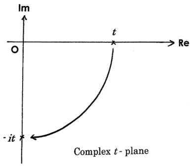
Figure 1. Fromrealtime$t$toimaginary$time-it$

a

heuristic path integral

(2.6) $\psi(t,x)=\int_{R^{d}}K(t,x;s,y)\psi(s,y)dy=\int_{\{X:X(t)=x\}}e^{iS(X)/\hslash}\psi(s,X(s))\mathcal{D}[X]$.

Next,

one

should know that$\mathcal{D}[X]$itself doesnotin general existin this situation

as

a

countably

additive

measure.

Therefore

we

cannot go further. But if we rotate in complex t-plane by

$-90^{0}:tarrow-it$ _(real time $t$ to imaginary time -it), i.e. if

we

go from

our

Minkowski

space-time to Euclidian space-time (see Figure 1), the situation changes. Before actually doing it,

for simplify put$\hslash=1$ and$s=0$

.

Then

our

(real-time) Schr\"odingerequation (2.1)

goes

tothe

imaginary-time Schr\"odingerequation, i.e. heatequation [formallyputting$u(t,x):=\psi(-it,x)$]

(2.7) $\frac{\partial}{\partial t}u(t,x)=[\frac{1}{2m}\Delta-V(x)]u(t,x)$, _$t>0$, $x\in R^{d}$

.

Simultaneously, theaction$S(X)$ in(2.3) changestointegralof theHamiltonian, and

so

$iS(X)$ to

time integral of the$Hamiltonian-\int_{0}^{t}[\frac{1}{2m}\dot{X}(\tau)^{2}+V(X(\tau))]d\tau$

.

Then_$K(t,x;0,y)$changes_to

(2.8) $K^{E}(t,x;0,y)= \int_{\{X;X(0)=y,X(t)=x\}}e^{-\int_{0}^{t}[\frac{1}{2m}X(\tau)^{2}+V(X_{0}(\tau))]d\tau}\mathcal{D}[X]$,

where the superscript $E$” is attributed to ”Euclideian”, and $K^{E}(t,x;0,y)$ should become the

(6)

fomula,

we

put here$X_{0}(\tau)$ $:=X(t-\tau),$ $0\leq\tau\leq t$, to transform paths$X(\cdot)$ topaths $X_{0}(\cdot)$ and

then getfrom(2.8)

(2.9) $K^{E}(t,x;0,y)= \int_{\{X:X_{0}(0)=x,\eta(t)=y\}}e^{-\int_{0^{[}\varpi^{\dot{\eta}(\tau)^{2}+V(\eta(\tau))]d\tau}}^{t1}}\mathcal{D}[X_{0}]$,

so

thatthe solution of(2.6) should begivenby the following pathintegral

(2.10) $u(t,x)= \int_{R^{d}}K^{E}(t,x;0,y)g(y)dy=\int_{\{X:X_{0}(0)=x\}}e$

‘_{$\int_{0\pi 0\mathfrak{v}_{g(X_{0}(t))\mathcal{D}[X_{0}]}}^{t1}[\dot{X}(\tau)^{2}+V(X(\tau))]d\tau$}

.

Remarkable is that N. Wiener, already around 1923, had constructed

a

countably additive

measure

$\mu_{x}(X_{0})$,for each$x\in R^{d}$,

on

the

space

$C_{x};=C_{x}([0,\infty)arrow R^{d})$ of thecontinuouspaths

(Bmwnian motions) $B:[0,\infty)arrow R^{d}$ startingffom_$B(O)=x$at time_$t=0$. This$\mu_{x}(\cdot)$iscalled

Wienermeasure,which is

a

probability

measure

on

$C_{0}$withcharacteristicfunction

$\exp[-t\frac{\xi^{2}}{2m}]=\int_{C_{X}([0,\infty)arrow R^{d})}e^{iB(t)\xi}d\mu_{x}(B)$

.

Around 1947, MarkKac, who had been at Comell University

as

Feynman and seemedto

haveheard his lecture, used the Wiener

measure

torepresentthe solution$u(t,x)$of theCauchy

problemof the heatequation(2.6)withinitial data$u(O,x)=f(x)$

as

a

genuine functional integral

(2.11) $u(t,x)= \int K^{E}(t,x;0,y)f(y)dy=\int_{C_{x}([0,\infty)arrow R^{d})}e^{-\int_{0}^{t}V(B(s))ds}f(B(t))d\mu_{x}(B)$.

This is the Feynman-Kac

_formula

[K66,80] alreadymentioned above. Thus, identify the path

$X_{0}(\cdot)$ appearing

on

the right-hand side of$(2.9)/(2.10)$with the continuouspath$B(\cdot)$ in$C_{x}$, then

theWiener

measure

$\mu_{x}(\cdot)$ tums out tobe constructed from the factor

“$e^{-\int_{0R^{B(\tau)^{2}d\tau}}^{t1}}\mathcal{D}[B]$”

on

theright-hand side of$(2.9)/(2.10)$

.

\S 3. Three MagneticRelativisticSchr\"odingerOperators

Weconsiderthequantized operator$H:=H_{A}+V$correspondingtothe classical Hamiltonian

(3.1) $\sqrt{(\xi-A(x))^{2}+m^{2}}+V(x)$, $(\xi,x)\in R^{d}\cross R^{d}$,

for

a

relativistic particle of

mass

$m$ under magnetic vectorpotential $A(x)$ and electric scalar

potential $V(x)$

.

This $H$ is used for

a

spinless particle in electromagnetic fields in the situation

where

we

may

ignore quantum-field theoretic effect like particlescreation and annihilation but

should take relativistic effectintoconsideration.

Inthisnote,

we

pay attentionto thefollowingthree quantizedoperators$H^{(1)},$ $H^{(2)}$ and$H^{(3)}$

correspondingtotheclassicalrelativisticHamiltonian symbol (3.1). Their difference is inhow

todefine the firstterm

on

theright,$H_{A}$,correspondingtothe symbol $\sqrt{(\xi-A(x))^{2}+m^{2}}$

.

For simplicity, it isassumed here and throughoutthis notethat$A(x)$ is smooth and $V(x)$ is

(7)

Definition3.1. The first $H^{(1)}$ _{$:=H_{A}^{(1)}+V$} is defined with

the first term

on

the right$H_{A}^{(1)}$

being the Weyl pseudo-differential operator through mid-pointprescription (e.g. [ITa86, I89,

I95]$)$

:

$(H_{A}^{(1)}f)(x):= \frac{1}{(2\pi)^{d}}\int\int_{R^{d}\cross R^{d}}e^{i(x-y)\cdot\xi\sqrt{(\xi-A(\frac{x+y}{2}))^{2}+m^{2}}f(\mathcal{Y})d_{\mathcal{Y}}d\xi}$

(3.2) $= \frac{1}{(2\pi)^{d}}\int\int_{R^{d}\cross R^{d}}e^{i(x-y)\cdot(\xi+A(\frac{x+y}{2}))}\sqrt{\xi^{2}+m^{2}}f(y)dyd\xi$

Definition

3.2.

The second $H^{(2)}$ _{$:=H_{A}^{(2)}+V$} is defined with

term$H_{A}^{(2)}$ being the

pseudo-differential operatormodified by Iftimie$-M\dot{a}ntoiu$-Purice_{$[IfMP07],$ $[IfMP08],$ $[IfMP10]$}:

(3.3) $(H_{A}^{(2)}f)(x):= \frac{1}{(2\pi)^{d}}\int\int_{R^{d}\cross R^{d}}e^{i(x-y)\cdot(\xi+\int_{0}^{1}A((1-\theta)x+\theta y)d\theta)}\sqrt{\xi^{2}+m^{2}}f(y)dyd\xi$.

Here the integralsin (3.2), (3.3)

on

the right-hand side

are

oscillatory integrals with$f$being

a

functionin$C_{0}^{\infty}(R^{d})$

or

in$S(R^{d})$

.

Definition3.3. The third $H^{(3)}$ _{$:=H_{A}^{(3)}+V$} is defined with _term$H_{A}^{(3)}$ being the

square

root

of the nonnegative selfadjointoperator$(-i\nabla-A(x))^{2}+m^{2}$

:

(3.4) $H_{A}^{(3)}:=\sqrt{(-i\nabla-A(x))^{2}+m^{2}}+V(x)$.

This$H_{A}^{(3)}$ does not seemto bedefined

as a

pseudo-differential operator corresponding to

a

certain tractablesymbol. So long

as

itis defined through Fourierandinverse-Fouriertansforms,

thecandiadte of its symbolwill notbe $\sqrt{(\xi-A(x))^{2}+m^{2}}$.

The last $H^{(3)}$ is used, for instance, to

study “stability of matter” in relativistic quantum

mechanics inE. Lieband R. $Se\ddot{m}nger$[LSei10].

Needles to say,

we can

show these three relativistic Schr\"odinger operators $H^{(1)},$ $H^{(2)}$ and

$H^{(3)}$ define selfadjoint operators in _{$L^{2}(R^{d})$}_, which

are

bounded from below and, in general,

different from

one

another. Infactfurther, thethree magnetic relativistic Schr\"odingeroperators

$H_{A}^{(1)},$$H_{A}^{(2)}$ and$H_{A}^{(3)}$

are

bounded from below by the samelowerbound

$m$

.

This

was

shown for

$H_{A}^{(1)}$ in [I89] with the aid ofits expression (5.5)in \S 5 instead of(3.2) andsimilarly

can

be for

$H_{A}^{(2)}$ withtheaidof(5.15)instead of(3.3), whileitis trivial for$H_{A}^{(3)}$

.

\S 4. GaugeCovariancefor Magnetic Relativistic Schrodinger Operators

Among these threemagneticrelativistic Schr\"odingeroperators$H_{A}^{(1)},$$H_{A}^{(2)}$ and$H_{A}^{(3)}$,the Weyl

quantized

one

like$H_{A}^{(1)}$ (in general, the Weyl pseudo-differential operator) is compatible well

with path integral. But it is pity that, for general vector potential $A(x)$ it is in general not

covariantunder

gauge

transformation,namely, thereexists

a

real-valued function$\varphi(x)$for which

(8)

However, $H_{A}^{(2)}$ (and

so

$H^{(2)}$)and$H_{A}^{(3)}$ (and

so

$H^{(3)}$)

are

gauge-covariant, though these three

are

notequalingeneral. Let

us

observe these factsinthe following.

First, why$H_{A}^{(3)}=\sqrt{(-i\nabla-A(x))^{2}+m^{2}}$ is

gauge-covariant

is because the selfadjoint

oper-ator $(-i\nabla-A(x))^{2}+m^{2}$ inside $\sqrt{}$

is

gauge-covariant. Next,

as

in the following

proposition,

it is

easy

to show that the modified$H_{A}^{(2)}$ is gauge-covariant. This property

was

emphasized in

$[IMP07],$ $[IfMP08],$ $[IfMP10]$ incontrastto$H_{A}^{(1)}$

.

Proposition

4.1.

$\mathscr{A}_{A}^{2)}$ iscovariantunder gaugetransformation, $i.e$

.

it

followss

for

any$\varphi\in$

$S(R^{d})$that$H_{A+\nabla\varphi}^{(2)}=e^{i\varphi}H_{A}^{(2)}e^{-i\varphi}$

.

Therefore,

so

is$H^{(2)}$

.

Theproof is duetothe

mean

value theorem.

Theorem

4.2.

$IfA(x)$is linear in$x,$ $i.e$

.

$\iota fA(x)=A\cdot x$with$A$beingany$d\cross d$real symmetric

constantmatrix, then$H_{A}^{(1)},$$H_{A}^{(2)}$and$H_{A}^{(3)}$coincide. Inparticular, this holds

for uniform

magnetic

fieldsfor

$d=3$

.

Proof is omitted.

\S 5. Imaginary-TimePathIntegrals forMagneticRelativistic Schrodinger Operators

Now, let $H$ be

one

of the magnetic relativistic Schr\"odinger operators $H^{(1)},$ $H^{(2)},$ $H^{(3)}$ in

Definitions 3.1, 3.2, _3.3. In the

same

way

as

in the nonrelativistic case, start ffom (real-time)

relativistic Schr\"odingerequation $i \frac{\partial}{\partial t}\psi(t,x)=H\psi(t,x)$

.

Rotateit by-90’ from real time $t$ to

imaginary$time-it$in complex t-plane,

we

amive

atthe

imaginary-time

relativistic Schr\"odinger

equation,

“heatequation” for$H-m$[formallyputting$u(t,x):=\psi(-it,x)$]: (5.1) $\{\begin{array}{ll}\frac{\partial}{\partial t}u(t,x)=-[H-m]u(t,x), t>0,u(O,x)=g(x), x\in R^{d}.\end{array}$

Thesemigroup$u(t,x)=(e^{-t[H-m]}g)(x)$givesthesolution of this Cauchyproblem. We want

to deal with path integral representation foreach $e^{-[H^{(j)}-m]}g(j=1,2,3)$

.

_The _{relevant path}

integral isconnectedwith theLe$vy$pmcess $[IkW81,89; Ap09]$

on

thespace$D_{x}:=D_{x}([0, \infty)arrow$ $R^{d})$of the “c\‘adlagpaths”,i.e. right-continuous paths$X:[0,\infty)arrow R^{d}$ having left-handlimits,

and with$X(O)=x$

.

_The associated path

space

measure

is

a

probability

measure

$\lambda_{x}$, for each

$x\in R^{d}$,

on

$D_{x}([0,\infty)arrow R^{d})$ whosecharacteristic function is givenby

(5.2) $e^{-t[\sqrt{\xi^{2}+m^{2}}-m]}= \int_{D_{X}([0,\infty)arrow R^{d})}e^{i(X(t)-x)\cdot\xi}d\lambda_{x}(X)$, $t\geq 0$, $\xi\in R^{d}$

.

We

are

going to start

on

task of representing the semigroup $e^{-t[H-m]}g$ by path integral.

(9)

heuristically in the present relativistic

case

(cf.[I93,

_pp.

26-29, \S 5]), to

compare

it with the

nonrelativistic

case

$(2.9)/(2.10)$, which together with $(2.2)/(2.6)$ is called configumtion space

path integml. Though taking the

same

procedure

as

beforeto findit,

we

tum outto leamitto

begivenby phasespacepath integml.

However, to

see

it,

_as

_{the general}

_case

_for$H$is dependent

on

whichof the three

relativis-tic Schr\"odinger operators is dealt with,

_{so we}

do only with the

case

$H_{0}$ $:=\sqrt{-\Delta+m^{2}}+V(x)$

withoutvectorpotential$A(x)$

.

Then

we

havefor the solution of(5.1)with$H_{0}$ inplaceof$H$

$u(t,x)=(e^{-t[H_{0}-m]}g)(x)$

(5.3) $= \int\int 0_{X(0)=x\}}^{t}$ .

Here$D[P]\mathcal{D}[X]$ $:= \prod_{0\leq\tau\leq t}\frac{dP(\tau)dX(\tau)}{(2\pi)^{d}}$ is

a

‘measure’

on

the spaceofthephasespacepaths(i.e.

momentum andpositionpaths) $(P,X);[0,t]\ni s\mapsto(P(s),X(s))\in R^{d}\cross R^{d}$ _with_$X(O)=x$ _and,

foreach fixed$\tau,$ $dP(\tau)dX(\tau)$is the Lebesgue

measure on

$R^{2d}=R^{d}\cross R^{d}$

.

Itwill tum outthat

the

measure

$\lambda_{x}(\cdot)$istobeconstmcted from the factor

$( \int_{\{P:arbitary\}}e^{-\int_{0}^{t}\{iP(s)dX(s)+[\sqrt{P(s)^{2}+m^{2}}-m]ds\}}\mathcal{D}[P])\mathcal{D}[X]$”

on

theright-hand side of(5.3),

so

that

we

have

a

correctfunctional integralrepresentaion quite

similar to the nonrelativistic

case

(2.11):

(5.4) $u(t,x)=(e^{-t[H_{0}-m]}g)(x)= \int_{D_{x}([0,\infty)arrow R^{d})}e^{-\int_{0}^{t}V(X(s))ds}g(X(t))d\lambda(X)$

.

Now

we

tum to

come

tothe situationinvolving also thevectorpotential$A(x)$

.

(1)First consider the

case

for the Weyl pseudo-differential operator$H^{(1)}=H_{A}^{(1)}+V$ in

Def-inition 3.1. The part$H_{A}^{(1)}$

can

berewritten

as

the integral operator:

$([H_{A}^{(1)}-m]f)(X)=- \int_{|y|>0}\tau$ .

$=- \lim_{r\downarrow 0}\int_{|y|\geq r}[e^{-iy\cdot A(x+\not\in)}f(x+y)-f(x)]n(dy)$

(5.5) $=-$

p.v.

$\int|y|>0^{[e^{-iy\cdot A(x+^{y})}}zf(x+y)-f(x)]n(dy)$

.

Here$n(dy)=n(y)dy$is

an

m-dependent

measure on

$R^{d}\backslash \{0\}$,calledL\’evymeasurewith density

(10)

$n(dy)$

appears

in

the L\’evy-Khinchin

formula:

(5.7) $\sqrt{\xi^{2}+m^{2}}-m=-\int_{|y|>0}[e^{iy\cdot\xi}-1-i\xi\cdot yI_{\{|y|<1\}}]n(dy)=-\lim_{rarrow 0+}\int_{|z|\geq r}[e^{iz\cdot\xi}-1]n(dz)$

.

Pmofof

(5.5). By the L\’evy-Khinchinformula(5.7),

$(H_{A}^{(1)}f)(x)=(2 \pi)^{-d}\int\int e^{i(x-y)\cdot(\xi+At^{x}\not\simeq^{+}))(m-\lim_{rarrow 0+}\int_{|z|\geq r}[e^{iz\cdot\xi}-1]n(dz))f(y)dyd\xi}$

$=(2 \pi)^{-d}[m\int\int e^{i(x-y)\cdot\xi}e^{i(x-y)\cdot A(^{X}\not\simeq^{+})}dyd\xi$

$- \lim_{rarrow 0+}\int\int\int_{|z|\geq r}(e^{i(x-y+z)\cdot\xi}-e^{i(x-y)\cdot\xi})n(dz)e^{i(x-y)\cdot At^{X}\not\simeq^{+})}f(y)dyd\xi]$

$=m \int\delta(x-y)e^{i(x-y)\cdot At^{x}\not\simeq^{+})}f(y)dy$

$- \lim_{rarrow 0+}\int\int_{|z|\geq r}(\delta(x-y+z)-\delta(x-y))n(dz)e^{i(x-y)\cdot A(^{X}\not\simeq^{+})}f(y)dy$

$=mf(x)- \lim_{rarrow 0+}\int\int_{|z|\geq r}(e^{-iz\cdot A(x+\xi)}f(x+z)-f(x))n(dz)$

.

$\square$

Torepresent$e^{-t[H^{(1)}-m]}g$ by path integral,

we

need

some

further notations from L\’evy

pro-cess.

For each path$X(\cdot),$ $N_{X}$(dsdy)denotesthecounting

measure on

$[0,\infty)\cross(R^{d}\backslash \{0\})$to count

the number ofdiscontinuiiesof$X(\cdot)$,i.e.

(5.8) $N_{X}((t,t’]\cross U):=\#\{s\in(t,t’];0\neq X(s)-X(s-)\in U\}$,

where$0<t<t’$and$U\subset R^{d}\backslash \{0\}$is

a

Borel set. Itsatisfies$\int_{D_{X}}N_{X}(dsdy)d\lambda_{x}(X)=dsn(dy)$

.

Put

$\overline{N}_{X}(dsdy)$ _{$:=N_{X}(dsdy)-dsn(dy)$},which

may

be thought of

as a

renormalization of$N_{X}(dsdy)$

.

Then

any

path$X\in D_{x}([0,\infty)arrow R^{d})$

can

beexpressedwith$N_{x}(\cdot)$and$\overline{N}_{X}(\cdot)$

as

(5.9) $X(t)=x+ \int_{0}^{t+}\int_{|y|\geq 1}yN_{X}(dsdy)+\int_{0}^{t+}\int_{0<|y|<1}y\overline{N}_{X}(dsdy)$

.

Now

we

havethe following path integralrepresentation for$e^{-t[H^{(1)}-m]}g$

.

Theorem

5.1

([ITa86], [I95]).

(11)

$S^{(1)}(t,X)=i \int^{t+}\int A(X(s-)+\frac{y}{2})\cdot yN_{X}(dsdy)+i\int^{t+}\int A(X(s-)+\frac{y}{2})\cdot y\overline{N}_{X}$_(dsdy)

(5.10) $+i \int_{0}^{t}ds$

p.v.

_{$\int_{0<|y|<1}A(X(s)+\frac{y}{2})\cdot yn(dy)+\int_{0}^{t}V(X(s))ds$}.

Pmof.

We onlygive

a

sketch. Put

(5.11) $(T(t)g)(x):= \int_{R^{d}}e^{-iA(^{x}\not\simeq^{+})\cdot(y-x)-V(X}\not\simeq^{+})t$ ,

where$k_{0}(t,x-y)$ istheintegral kemel of$e^{-t(\sqrt{-\Delta+m^{2}}-m)}$. Then

we

can

rewriteit

as

$(T(t)g)(x)= \int_{D_{x}}e^{-iA(\frac{x+X(t)}{2})\cdot(X(t)-x)-V(\frac{x+X(t)}{2})t}g(X(t))d\lambda_{x}(X)$

withpartitionof$[0,t]:0=t_{0}<t_{1}<\cdots<t_{n}=t,$ $t_{j}-t_{j-1}=t/n$,

(5.12) $S_{n}(x0, \cdots,x_{n}):=i\sum_{j=1}^{n}A(\frac{x_{j-1}+x_{j}}{2})\cdot(x_{j}-x_{j-1})+\sum_{j=1}^{n}V(\frac{x_{j-1}+x_{j}}{2})\frac{t}{n}$,

where$x_{j}=X(t_{j})(j=0,1,2, \ldots,n);x=x_{0}=X(t_{0}),$ $y=x_{n}=X(t_{n})\equiv X(t)$

.

Substitute these$n+1$ pointsof path$x_{j}=X(t_{j})$into$S_{n}(x_{0}, \cdots,x_{n})$to get

$S_{n}(X):=S_{n}(X(t_{0}), \cdots,X(t_{n}))$ $=i \sum_{j=1}^{n}A(\frac{X(t_{j-1})+X(t_{j})}{2})\cdot(X(t_{j})-X(t_{j-1}))+\sum_{j=1}^{n}V(\frac{X(t_{j-1})+X(t_{j})}{2})\frac{t}{n}$ Then $n$times $= \int_{D_{x}}e^{-S_{n}(X)}g(X(t))d\lambda_{x}(X)$. We

can

show

Proposition

5.2.

$T(t/n)^{n}garrow e^{-t[H^{(1)}-m]}g$ _in $L^{2}(R^{d})$, $narrow\infty$

.

Proofisomitted.

Now

we are

in

a

positiontocomplete the proof of Theorem

5.1.

By Proposition 5.2,

we

see

theleft-hand side of(5.13) converges to$e^{-t[H^{(1)}-m]}g$

as

_{$narrow\infty$}

.

On the_{other hand,}

we see

_by

$It\hat{o}$’s formula [$see*)$ below] that theright-hand side

converges

to

$\int_{D_{x}}e^{-S(X)}g(X(t))d\lambda_{x}(X)$ by

(12)

$*)$

Forinstance,in $t_{j-1}\leq s<t_{j}$,

we

havebyIt\^o’s formula,

$A( \frac{X(t_{j-1})+X(t_{j})}{2})\cdot(X(t_{j})-X(t_{j-1}))$

$= \int_{t_{j}-1}^{t_{j}+}\int_{|y|>0}[A(\frac{X(s-)+X(t_{j-1})+yl_{|y|\geq 1}(y)}{2})\cdot(X(s-)-X(t_{j-1})+yI_{|y|\geq 1}(y))$

$-A( \frac{X(s-)+X(t_{j-1})}{2})\cdot(X(s-)-X(t_{j-1}))]N_{X}(dsdy)$ $+ \int_{t_{j}-1}^{t_{j}+}\int_{|y|>0}[A(\frac{X(s-)+X(t_{j-1})+yI_{|y|<1}(y)}{2})\cdot(X(s-)-X(t_{j-1})+yI_{|y|<1}(y))$ $-A( \frac{X(s-)+X(t_{j-1})}{2})\cdot(X(s-)-X(t_{j-1}))]\overline{N}(dsdy)$ $+ \int_{t_{j}-1}^{t_{j}}\int_{|y|>0}[A(\frac{X(s)+X(t_{j-1})+yI_{|y|<1}(y)}{2})\cdot(X(s)-X(t_{j-1})+yI_{|y|<1}(y))$ $-A( \frac{X(s)+X(t_{j-1})}{2})\cdot(X(s)-X(t_{j-1}))$ $-I_{|y|<1}(y) \{(\frac{1}{2}(y\cdot\nabla)A)(\frac{X(s)+X(t_{j-1}}{2})\cdot(X(s)-X(t_{j-1}))$

$+y \cdot A(\frac{X(s)+X(t_{j-1})}{2})\}]dsn(dy)$.

(2) Next

we

come

to the

case

for the pseudo-differential operator modified by

Iftimie-Mantoiu-Purice: $H^{(2)}:=H_{A}^{(2)}+V$ in Definition 3.2. By exactly the

same

argument

as

usedto

show (5.5),

we can

showthat

$([H_{A}^{(2)}-m]f)(x)=- \int_{|y|>0}[e^{-iy\cdot\int_{0}^{1}A(x+\theta y)d\theta}f(x+y)-f(x)$

$-I_{\{|y|<1\}}y\cdot(\nabla-iA(x))f(x)]n(dy)$

$=- \lim_{r\downarrow 0}\int_{|y|\geq r}[e^{-iy\cdot\int_{0}^{1}A(x+\theta y)d\theta}f(x+y)-f(x)]n(dy)$

(5.13) $=-$p.v.$\int_{|y|>0}[e^{-iy\cdot\int_{0^{1}}A(x+\theta y)d\theta}f(x+y)-f(x)]n(dy)$.

Theorem

5.3.

$[ImP07, IfMP08, IfMP10]$

$(e^{-t[H^{(2)}-m]}g)(x)= \int_{D_{X}([0,\infty)arrow R^{d})}e^{-S^{(2)}(t,X)}g(X(t))d\lambda_{x}(X)$,

$S^{(2)}(t,X)=i \int_{0}^{t+}\int_{|y|\geq 1}(\int_{0}^{1}A(X(s-)+\theta y)\cdot yd\theta)N_{X}(dsdy)$

$+i \int_{0}^{t+}\int_{0<|y|<1}(\int_{0}^{1}A(X(s-)+\theta y)\cdot yd\theta)\overline{N}_{X}(dsdy)$

(5.14) $+i \int_{0}^{t}ds$p.v.$\int_{0<|y|<1}(\int_{0}^{1}A(X(s)+\theta y)\cdot yd\theta)n(dy)+\int_{0}^{t}V(X(s))ds$.

The proof of Theorem5.3 will be done in exactly the

same

way

as

that ofTheorem 5.1.

(13)

(3)Finally,

we

considerthe

case

forthe operatordefined, inDefinition 3.3, with the

square

rootof

a

nonnegative selfadjointoperator,$H^{(3)}$ _{$:=H_{A}^{(3)}+V$}

.

On the

one

hand,

we can

determine by functional analysis, namely, by theory of fractional

powers

(e.g. [Y68,Chap.IX,11,pp.259-261])$e^{-t[H_{A}^{(3)}-m]}$

fromthe nonnegative selfadjoint

op-erator$S:=(-i\nabla-A(x))^{2}+m^{2}=:2mH_{A}^{NR}+m^{2}$ _where$H_{A}^{NR}$ stands for the magnetic

nonrela-tivisticSchr\"odingeroperator $\frac{1}{2m}(-i\nabla-A(x))^{2}$without scalar potential. Indeed,

we

have

$e^{-t[H_{A}^{(3)}-m]}g=\{\begin{array}{ll}e^{mt}\int_{0}^{\infty}f_{t}(\lambda)e^{-\lambda S}gd\lambda, t>0,0, t=0\end{array}$

(5.15) $f_{t}(\lambda)=\{\begin{array}{ll}(2\pi i)^{-1}\int_{\sigma-i\infty}^{\sigma+i\infty}e^{z\lambda-tz^{1/2}}dz, \lambda\geq 0,0, \lambda<0 (\sigma>0).\end{array}$

Here

we

quickly insert the $Feynman-Kac$-It\^o

_formula

(e.g. [S05]) for the magnetic

non-relativistic Schr\"odingeroperator$H^{NR}$ _{$:=H_{A}^{NR}+V$}_{$:= \frac{1}{2m}(-i\nabla-A(x))^{2}+V(x)(m>0)$}_,a

more

generalformula than the Feynman-Kac formula(2.11):

(5.16) $(e^{-tH^{NR}}g)(x)$

$= \int_{C_{x}([0,\infty)arrow R^{d})}e0z^{i}g(B(t))d\mu_{x}(B)$

$\equiv\int_{C_{x}(l0,\infty)arrow R^{d})^{e^{-[i\int_{0}^{t}A(B(s))odB(s)+\int_{0}^{t}V(B(s))ds]}}}g(B(t))d\mu_{x}(B)$.

This

can

provide

a

kindof pathintegral representationfor$e^{-t[H_{A}^{(3)}-m]}g$_{with the}_Wienermeasure,

by substituting the$Feynman-Kac$-It\^o formula(5.17) for$V=0$with$t=2m\lambda$into$e^{-t(S-m^{2})}j=$

$e^{-2m\lambda H_{A}^{NR}}$

in the integrand of equation(5.16) for$e^{-t[H_{A}^{(3)}-m]}g$

.

_Then, _to _represent$e^{-t[H^{(3)}-m]}g$

for$V\neq 0$,

we

might applytheTrotter-Kato product formula

(5.17) $e^{-t[H^{(3)}-m]}= s-\lim_{narrow\infty}(e^{-(t/n)[H_{A}^{(3)}-m]}e^{-(t/n)V})^{n}$,

tothesum$H^{(3)}-m=(H_{A}^{(3)}-m)+V$ _to

express

_the semigroup$e^{-t[H^{(3)}-m]}$ as a_“limit”, _where

convergence

ofthe right-hand side usually takes place in strong

sense as

indicated, but

now

even, in operator norm, by therecent results

on

operator

norm

convergence [ITOI], [ITTZOI] (cf. [IT04], [IT06]). However itisnotclear whether this procedure couldfurther yield

a

path

integralrepresentation for$e^{-t[H^{(3)}-m]}g$

.

On the other hand, it does not

seem

possible to represent $e^{-t[H^{(3)I}-m]}g$ _{by path integral}

through directly applyingL\’evyprocess,

as we saw

inthe

cases

for$e^{-t(H^{(1)}-m)}g$and$e^{-t(H^{(2)}-m)}g$_,

because$H_{A}^{(3)}$ doesnot

seem

tobe explicitly expressed by

a

pseudo-differentialoperatorof

a

cer-taintractable symbol. It

was

in this situation thattheproblem of path integral representationfor

$e^{-t[H^{(3)\mathfrak{l}}-m]}g$

was

studied first by DeAngelis-Serva

and Rinaldi $[AnSe90, AnRSe91]$ with

use

(14)

not onlyforthemagnetic relativisticSchr\"odinger operator$H_{A}^{(3)}$ butalso for Bemstein functions

of the magnetic nonrelativisticSchr\"odinger operator

even

with spin. To proceed, let

us

explain

aboutsubordination.

Let$B^{1}(t)$be theone-dimensional standard Brownianmotionbeing

a

functionin$C_{0}([0,\infty)arrow$

R$)$ with$B^{1}(0)=0$,

so

that $e^{-t_{T}^{\mathcal{E}^{2}}}= \int_{C_{0}([0,\infty)arrow R)}e^{i\xi B^{1}(t)}d\mu_{0}^{1}(B^{1})$ with$\mu_{0}^{1}$ theWiener

measure on

$C_{0}([0,\infty)arrow R)$

.

Put

(5.18) $T(t)$ $:= \inf\{s>0 ; B^{1}(s)+\sqrt{m}s=\sqrt{m}t\}$, $t\geq 0$

.

Then $T(t)$ is

a

monotone, non-decreasing function

on

$[0,\infty)$ with $T(O)=0$, belonging to

$D_{0}([0, oo)arrow R)$ and

so

becoming

a

one-dimensionalL\’evyprocess, calledsubordinator. Let $v0$

bethe associated probability

measure on

$D_{0}([0,\infty)arrow R)$

.

Proposition

5.4.

(e.g. [Ap09, p.54,Example 1.3.21])

(5.19) $e^{-t[\sqrt{2m\sigma+m^{2}}-m]}= \int_{D_{0}([0,\infty)arrow R)}e^{-T(t)\sigma}dv_{0}(T)$, $\sigma\geq 0$.

Thisproposition implies that thechacteristic functionof the

measure

$v_{0}$ is givenby

$e^{-t\phi(p)}= \int_{D_{0}([0,\infty)arrow R)}e^{iT(t)\rho}dv_{0}(T)$, $\rho\in R$,

$\phi(p)=(\frac{m}{2})^{1/2}\frac{\sqrt{m^{2}+\rho^{2}}-m}{(\sqrt{m^{2}+\rho^{2}}+m)^{1/2}+\sqrt{2}m^{1/2}}-\frac{(2m)^{1/2}\rho}{(\sqrt{m^{2}+\rho^{2}}+m)^{1/2}}i$

.

To

see

this,first analytically extend$\sqrt{2m\sigma+m^{2}}$tothe right-half complex plane_{$z:=\sigma+i\rho,$} _$\sigma>$

$0,\rho\in R$, and then

we

have $\phi(p)=\lim_{crarrow+0}\sqrt{2m(\sigma+i\rho)+m^{2}}-m$_, of which the right-hand

side is calculated

as

above.

We

are

in

a

position togive

a

pathintegralrepresentationfor$e^{-t[H^{(3)}-m]}g$

.

Theorem

5.5.

$[AnSe90,$$AnRSe91$;HIL09$]$

$(e^{-t[H^{(3)l}-m]}g)(x)= \int\int_{C_{X}([0,\infty)arrow R^{d})}e^{-S^{(3)}(t,B,T)}g(B(T(t)))d\mu_{X}(B)dv_{0}(T)\cross D_{0}([0,\infty)arrow R)$’

$S^{(3)}(t,B, T)=i \int_{0}^{T(t)}A(B(s))dB(s)+\frac{i}{2}\int_{0}^{T(t)}divA(B(s))ds+\int_{0}^{t}V(B(T(s)))ds$,

(5.20) $\equiv i\int_{0}^{T(t)}A(B(s))\circ dB(s)+\int_{0}^{t}V(B(T(s)))ds$,

where$\mu_{x}$ isthe Wiener

measure

on$C_{x}([0,\infty)arrow R^{d})$

.

Proofof

Theorem5.5. (Sketch) We

use

Proposition 5.4and the$Feynman-Kac$-It\^oformula

(15)

operator$H_{A}^{NR}$ ,

we

have

$H_{A}^{NR}= \int_{Spec(H_{A}^{NR})}\sigma dE(\sigma)$

.

Then for$f,$$g\in L^{2}(R^{d})$

$\{f,e^{-t[H_{A}^{(3)}-m]}g\}=\int_{Spec(H_{A}^{NR})}e^{-t[\sqrt{2m\sigma+m^{2}}-m]}\{f,dE(\sigma)g\}$ ,

where $\{\cdot,$$\cdot\}$ standsfor the innerproductof the Hilbert

space

_{$L^{2}(R^{2})$}

.

By Propositopn 5.4 and

again by SpectralTheorem,

$\{f,e^{-t[H_{A}^{(3)}-m]}g\}=\int_{Spec(H_{A}^{NR})}\int_{D_{0}([0,\infty)arrow R)}e^{-T(t)\sigma}dv_{0}(T)\langle f,dE(\sigma)g\}$

$= \int_{D_{0}([0,\infty)arrow R)}\langle f,e^{-T(t)H_{A}^{NR}}g\rangle dvo(T)$

.

Applyingthe$Feynman-Kac$-It\^oformula(5.17) (with$V=0$)to$e^{-T(t)H_{A}^{NR}}g$ontheright,

we

_have

$\langle f,e^{-t[H_{A}^{(3)}-m]}g\rangle$

$= \int D_{0([0,\infty)arrow R)^{v0}}d(T)\int_{R^{d}}dx\overline{f(B(0))}\int_{C_{X}([0,\infty)arrow R^{d})}e^{-i\int_{0^{T(t)}}A(\beta(s))\circ dB(s)}g(B(T(t)))d\mu_{x}(B)$

$= \int_{R^{d}}d_{X}\overline{f(x)}\int\int_{\cross D_{0}([0,\infty)arrow R)}C_{x}(l0,\infty)arrow R^{d})^{e^{-i\int_{0^{T(t)}}A(B(s))\circ dB(s)}}g(B(T(t)))d\mu_{x}(B)d|nu_{0}(T)$ ,

wherenote$B(O)=x$

.

Thisproves theassertionwhen$V=0$

.

When $V\neq 0$, with partition of _{$[0,t]:0=t_{0}<t_{1}<\cdots<t_{n}=t,$} _{$t_{j}-t_{j-1}=t/n$},

we

can

express

$e^{-t[H^{(3)}-m]}g=e^{-t[(H_{A}^{(3)}-m)+V]}$ _by_the_{Trotter-Kato formula}_(5.18). _Rewrite_the_product

of these $n$ operators by path integral with respect to the product oftwoprobability

measures

$vo(T)\cdot\mu_{x}(B)$ and note that_{$T(O)=T(t_{0})=0,$ $B(O)=B(T(t_{0}))=x$}_,then

we

have $\{f, (e^{-(t/n)[H_{A}^{(3)}-m]}e^{-(t/n)V})^{n}g\}$

$= \int_{R^{d}}dx\int_{D_{0}([0,\infty)arrow R)}dv_{0}(T)\int_{C_{x}([0,\infty)arrow R^{d})}\overline{f(B(0))}$

$\cross e^{-i\Sigma_{j=1}^{n}\int_{\tau t_{j-1})}^{T(t_{j})}A(B(s))\circ dB(s)_{e^{-\Sigma_{j=1}^{n}V(B(T(t_{j}))\frac{t}{n}}}}tg(B(t_{n}))d\mu_{x}(B)$

. Wesee,

as

$narrow\infty$,that theleft-hand sideconvergesto $\langle f,e^{-t[H_{A}^{(3)}-m]}g\rangle$

,andtheright-handside

also

converges

tothe goal formula by the Lebesguetheorem,

_as

integral by$dx\cdot v_{0}(T)\cdot\mu_{x}(B)$

.

Hence

or

similarly

we can

alsoget(5.21). $\square$

Finally,

as summary,

we

will collect the three path integralrepresentation formulas in

The-orems

5.1, 5.3, 5.5, below,

so as

tobe able toeasily

see

x-dependence. To do so, make change of

space,

probablity

measure

and paths by translation:

(16)

$D_{x}arrow D_{0},$ $\lambda_{x}arrow\Lambda_{0},$$X(s)arrow X(s)+x,$ $B(s)arrow B(s)+x,$ $B(T(s))arrow B(T(s))+x$, then

(5.10): $(e^{-\prime[H^{(1)}-m]}g)(x)= \int_{D_{0}([0,\infty)arrow R^{d})}e^{-S^{(1)}(t,X)}g(X(t)+x)dA_{0}(X)$,

$S^{(1)}(t,X)=i \int_{0}^{t+}\int_{|y|\geq 1}A(X(s-)+x+\frac{y}{2})\cdot yN_{X}$(dsdy)

$+i \int_{0}^{t+}\int_{0<|y|<1}A(X(s-)+x+\frac{y}{2})\cdot y\overline{N}_{X}(dsdy)$

$+i \int_{0}^{t}dsp.v.\int_{0<|y|<1}A(X(s)+x+\frac{y}{2})\cdot yn(dy)$

$+ \int_{0}^{t}V(X(s)+x)ds$;

(5.15): $(e^{-t[H^{(2)}-m]}g)(x)= \int_{D_{0}([0,\infty)arrow R^{d})}e^{-S^{(2)}(t,X)}g(X(t)+x)dA_{0}(X)$,

$S^{(2)}(t,X)=i \int_{0}^{t+}\int_{|y|\geq 1}(\int_{0}^{1}A(X(s-)+x+\theta y)\cdot yd\theta)N_{X}(dsdy)$

$+i \int_{0}^{t+}\int_{0<|y|<1}(\int_{0}^{1}A(X(s-)+x+\theta y)\cdot yd\theta)\tilde{N}_{X}(dsdy)$

$+i \int_{0}^{t}dsp.v.\int_{0<|y|<1}(\int_{0}^{1}A(X(s)+x+\theta y)\cdot yd\theta)n(dy)$

$+ \int_{0}^{t}V(X(s)+x)ds$;

(5.21): $(e^{-t[H^{(3)\mathfrak{l}}-m]}g)(x)= \int\int_{\cross D_{0}([0,\infty)arrow R)}C_{0}([0,\infty)arrow R^{d})e^{-S^{(3)}(t,B,T)}g(B(T(t))+x)d\mu_{0}(B)dv_{0}(T)$,

$S^{(3)}(t,B, T)=i \int_{0^{A(B(s)+x)\cdot dB(s)}}^{T(t)}+\frac{i}{2}\int_{0^{d}}^{T(t)}ivA(B(s)+x)ds$

$+ \int_{0}^{t}V(B(T(s))+x)ds$,

$\equiv i\int_{0}^{T(t)}A(B(s)+x)\circ dB(s)+\int_{0}^{t}V(B(T(s))+x)ds$

\S 6. Feynman andDirac

Finally, I would liketoclose thesnotes towrite somethingaboutFeynman and Dirac.

In \S 1,

we

observed Feynman’sTwo Postulatesequivalentto“path integral”. Inthem, _equation

(2.5) saying that $\varphi[X]$ is “proportional to” $e^{S(X)/\hslash}$ is the pivotal point. As he himselfwrote

(17)

([D33, D35], [D45])”, _{though. For what Dirac had criptically remarked}

_as

_{”analogous to”}

there,Feynmanbelievedtobe abletosubstitute”proportional to”(see Preface of[FH65]).

There has recently been published

a

book entitled The Strangest Man: The Hidden

_Life

of

Paul Dimc, Quantum Genius, by Graham Farmelo [Faber and Faber Ltd, London, 2009;

paperback ed. 2010]. This volume describes indetail the life of Dirac from his birthto death

with much favor and affection. From it I have leamed something novel which lets

me

think

again about how it

was

when Feynman had met Dirac, _{and how Feynman had been} _thinking

afterwards.

*Time: September

1946

*Place: Conference

on

’The Future of NuclearScience’, Princeton‘s Graduate College.

Feynman

was

Chairmantointroduce Diractothe audience. Thefollowing 12lines

are

cited

from this book by GrahamFarmelo,Chap. 24,

_p.

333.

FeynmandescribedinhispmblemtoDimc and

came

tocrunch:

FEYNMAN.$\cdot$ Didyou know

that they

were

pmpotional ?

DIRAC:Are they ?

FEYNMAN: Yes they

are.

DIRAC: That’s interesting.

Dirac thengotupand walkedaway. Feynman subsequentlybecame

_famousfor

his version

of

quantum mechanics but thought the credit

was

undeserved. The

more

closely he lookedat

the ’little paper‘, _the

_more

herealizedthathehaddone nothingnew. Helatersaid, repeatedly,

‘Idon’tknow what all

_thefu

ssis about–Dirac did it all

_before

me.’

[Intervie$w$withFreeman Dyson,27June2005. Dysonnoted thatFeynmanmade

thepointrepeatedly.]

References

[Ap09] Applebaum, D., Levyprocesses andStochastic Calculus, 2nd Ed., Cambridge University Press2009.

[BCSS85] Blanchard,Ph., Combe, Ph., Sirugue,M. and Simgue-CollinM.,Pathintegralrepresentation

for the solution of the Dirac equation inpresence ofanextemalelectromagnetic field,Path integmls

_from

meVto MeV(Bielefeld, 1985), Bielefeld Encount. Phys. Math., VII, World Sci.Singapore1986,pp. 396-413.

[CSS86] Combe, Ph.,Sirugue,M. and Simgue-CollinM.,Pointprocessesand quantumphysics: some

recent developments and results, VIIIth Imemational Congress on Mathematical Physics

(Marseille, 1986),WorldSci.Singapore 1987,pp. 421-430.

[AnRSe91] DeAngelis, G. F., Rinaldi A. and Serva, M., Imaginary-time pathintegral forarelativistic

spin-(1/2)particleinamagnetic field,_{Europhys. Lett.} ₁₄(1991),_95-100.

[AnSe90] DeAngelis, G. F. andServa, M.,On the relativistic Feynman-Kac-Itoformula,J. Phys. A23

(1990),_965-968.

(18)

6A72(1933).

[D35] –, The Principles

of

Quantum Mechanics, The Clarendon Press, Oxford, 1935, 2nd

Ed.,_Sec.33.

[D45] –, On the analogy between classical and quantum mechanics, Rev. Mod. Phys. 17

(1945), 195-199.

[F48] Feynman, R. P., Space-time approach to non-relativistic quantum mechanics, Rev. Mod.

Phys.,20(1948),_367-387.

[F05] Feynman’s Thesis–ANewApproachtoQuantum Theory,(Brown, L. M.,ed.), WorldSci.

2005,(includingFeynman‘sThesistogether with[F48], [D33]).

[FH65] Feynman, R. P. and Hibbs, A. P., Quantum Mechanics and Path Integmls, McGraw-Hill,

1965; AlsoEmendeded. byDaniel F. Styer, DoverPublications, Inc.Meneola, NewYork,

2005.

[HIL09] F.Hiroshima,T.Ichinose andJ.L\’orinczi : Pathintegral representationfor Schr\"odinger

oper-atorswithBemsteinfunctions of the Laplacian,Preprint2009.

[I82] T. Ichinose: Pathintegral fortheDirac equation intwospace-timedimensions, Pmc. Japan

Academy58A(1982),_290-293.

[I84] T. Ichinose: Path integralforahyperbolic system of the firstorder,Duke Math. J51(1984),

1-36.

[I89] T. Ichinose: Essential selfadjointness of the Weyl quantized relativistic Hamiltonian, Ann. Inst. H. Poincare, Phys. Theor51 (1989),_265-298.

[I93] T. Ichinose: Path integral for the Dirac equation, Sugaku Expositions, Amer. Math. Soc. 6

(1993), 15-31.

[I95] T. Ichinose: Some resultsonthe relativistic Hamiltonian: Selfadjointnessandimaginary-time

pathintegral,

_Differential

Equations and MathematicalPhysics, pp. 102-116,Intemational Press,Boston 1995.

[ITOI] T. Ichinose and Hideo Tamura: Thenormconvergenceof theTrotter-Katoproduct formula

with error bound, Commun. Math. Phys. 217 (2001), 489-502; Erratum Commun. Math.

Phys. 254(2005),No.1,255.

[IT04] T. Ichinose and Hideo Tamura: Sharp

error

boundon

norm

convergenceof exponential prod-uct formulaandapproximationtokemels ofSchr\"odingersemigroups, Comm. Partial

Differ-ential Equations29(2004),Nos. 11/12, 1905-1918.

[IT06] T. Ichinose and Hideo Tamura: Exponential product approximation to integral kemel of Schr\"odinger semigroup and to heat kemel ofDirichlet Laplacian, J Reine Angew Math.

592(2006), 157-188.

$[IT\Gamma Z01]$ T. Ichinose, HideoTamura, Hiroshi Tamura and V A.Zagrebnov: Note onthepaper “The

nolmconvergence of the Trotter-Kato product formulawitherrorbound”byIchinose and

Tamura,Comnun. Math. Phys. 221(2001),499-510.

[ITa84] T. Ichinose and HiroshiTamura: Propagation ofa Dirac particle-Apathintegral approach,

J. Math. Phys.25(1984), 1810-1819.

[ITa86] T. Ichinose and Hiroshi Tamura: Imaginary-timepathintegralforarelativistic spinless par-ticle inanelectromagnetic field,Commun. Math. Phys. 105(1986),239-257.

[ITa87] T. Ichinose and Hiroshi Tamura: Path integral approach torelativistic quantummechanics

-Two-dimensional Dirac equation, Supplement

_of

Progress

_of

Theoretical Physics No.92

(1987), 144-175.

[ITa88] T. Ichinose and HiroshiTamura: The Zitterbewegung ofaDiracparticle in two-dimensional space-time, J Math. Phys. 29(1988), 103-109.

(19)

Math. Sci.KyotoUniv. 43(2007),_585-623.

[IfMP08] V. Iftimie, _M. _Mtintoiu _and R. Purice: Estimating the number ofnegative eigenvalues of

a relativistic Hamiltonian with regular magnetic field, Topics in appliedmathematics and

mathematicalphysics,_{97-129, Ed. Acad. Rom\^ane,}Bucharest,_2008.

[IfMP10] V.Iftimie,M.$M\dot{a}ntoiu$andR. Purice:Unicity of theintegrateddensity of states for_relativistic

Schr\"odingeroperatorswithregular magnetic fields and singularelectricpotentials, Integml Equations OpemtorTheory7(2010), _215-246.

[IkW81,89] N. Ikeda and S.Watanabe: Stochastic

_Differential

Equationsand

_Diffusion

Processes,

North-HollandMathematicalLibrary, 24, North-Holland Publishing Co., Amsterdam; Kodansha, Ltd., Tokyo, 1981, 2nd ed. 1989.

[K66,80] _{M. Kac: Wiener}and integrationinfunctionspaces,Bull. Amer. Math. Soc.72,PartII(1966),

pp.52-68; Integration inFunctionSpaces andSome

_of

ItsApplications, LezioniFemiane, AccademiaNazionale delLincei ScuolaNorm.Sup.Pisa 1980.

[LSei10] _{E. H. Lieb and R.} Seiringer: The Stability

_of

Matter in QuantumMechanics, Cambridge

UniversityPress2010.

[S05] B. Simon:FunctionalIntegmtionand QuantumPhysics,2nded.,AMS Chelsea Publishing,

Providence, RI,2005.

[Y68] K. Yosida: Functionalanalysis, Springer-VerlagNew YorkInc.,NewYork,2nded. 1968.

[Z88] T. Zastawniak: Pathintegralsforthe telegrapher’s andDiracequations; the analytic family of

measures

and theunderlyingPoissonprocess,Bull. Polish Acad.Sci.M血論．36(1988),no.

5-6,_341-356(1989).

[Z89] T. Zastawniak: Pathintegralsfor the Dirac equation–some recent developmentsin math-ematical theory, StochasticAnalysis,PathIntegmtionandDynamics(Warwick, 1987),