Three-dimensional numerical simulation of the motion of a droplet on an inclined plane

Three-dimensional numerical simulation of the motion of a droplet on an inclined plane

N

T

C

Graduate School of Natural Science and Technology, Kanazawa University, Kakuma, Kanazawa, 920-1192, Japan (Received July 4, 2013 and accepted in revised form August 9, 2013)

Abstract This paper introduces a mathematical model represented by a system of equa- tions for a droplet moving on an inclined plane. A three-dimensional simulation for this phenomenon is obtained by solving a system of equations based on both discrete Morse flow and the smoothed particle hydrodynamics method.

Keywords. coupled model, free boundary, volume constraint, hyperbolic problem, droplet motion

1 Introduction

In this work, we derive a model for a moving droplet on a surface. The motion of droplet has been described by various models, in which it is usually difficult to model the dy- namical contact angle [10]. In our model, we consider a coupling of film representing the surface of the droplet and of fluid inside the film. Physical parameters of the film model such as surface tensions or velocity determine implicitly the contact angle. We assume that the fluid motion follows the Euler equations and that the film and fluid interact via pressure force. This leaves us with the problem of deriving a model for the motion of the film.

Surface tensions are important factors in describing the shape of droplets. For a liq- uid drop, there are three types of surface tensions: solid-surface tension γ

, the liquid- surface tension γ

and the solid-liquid interfacial surface tension γ

(Figure 1). In equilibrium, the contact angle of the droplet is determined by the properties of the liquid and the material on which the droplet is lying [16]. In particular, the relationship between the contact angle and the surface tensions is given by Young’s equation:

γ

− γ

= γ

cos θ .

∗Present address: Camau Teacher Training College, 155A, Nguyen Tat Thanh Street, Camau City, Viet- nam. e-mail: [email protected]

Figure 1: The setting of the model.

In our work, we focus only on the case where the dynamic contact angle θ ∈ [ 0 , 90

).

In this setting, we describe the shape of the film by a scalar function u . In addition, since the motion of the droplet is constrained by the surface over which it is moving, there appears an obstacle in our model equation. Moreover, as the droplet moves and changes its shape, we assume that the volume of the fluid is preserved.

To summarize, we develop a model for a film with positive contact angle under volume-constraint and an obstacle. The equation of motion for the film in this paper is obtained as the stationary point of the action integral for the system. The numerical solution of the model equation is obtained by the method of discrete Morse flow, which has been developed by N. Kikuchi to solve parabolic problems [5]. This method was also used to solve hyperbolic problems [2], [9], and one of the extensions of this method was used to solve free-boundary problems [3], [6], [10]. Solving volume-preserving prob- lems is another extension of this method [13], [12] and we remark that this method can naturally apply to the free boundary problems with volume constraint [14], [1].

For the fluid motion, we use the smoothed particle hydrodynamics method (SPH) to solve the Euler equations. The system of equations is then solved by the combination of both methods. Through this coupling approach, we are able to realize the dynamic contact angle in an implicit way, i.e., only through the consideration of the energy of the system. In this sense, we believe that this method can overcome the necessity of prescribing the contact angle evolution explicitly. This necessity causes difficulties in most of the existing models.

2 The model equations

In this section, we derive the model equation for the motion of a droplet on an inclined plane. Our model is described by a system of equations which consists of the governing equation for the motion of a film, together with the equation for the motion of fluid inside the film.

2.1 The equation of motion for the film

In this section, we examine the surface of the droplet. The equilibrium shape of the

droplet is our starting point. From our assumptions that the droplet can be described by

a scalar function, we express the evolution of the film by a function:

u : Ω × ( 0 , T ) −→

,

where ( 0 , T ) is the time interval and Ω ⊂

is the domain where the motion is consid- ered. The boundary of ∂ Ω is assumed to be Lipschitz on which a Dirichlet condition is prescribed and the film is assumed not to go under the plane. Moreover, the volume enclosed under the film is assumed to be constant, that is

Ω

u χ

dx = V > 0 . The surface energy of the stable droplet can thus be written as

E =

Ω

γ

1 + |∇u |

χ

dx +

Ω

γ

χ

dx , (2.1) where γ

= γ

and γ

= γ

− γ

.

If we assume that the minimizer exists and is smooth, we obtain the following result (see [11]).

Lemma 1.

Let the minimizer of (2.1) be smooth in { u > 0 }. Then Young’s equation γ

= −γ

cos θ

holds on ∂ { u > 0 }.

We rewrite equation (2.1) as follows:

E =

Ω

γ

1 + |∇u |

dx +

Ω

(γ

+ γ

)χ

dx − γ

|Ω|. (2.2) Now suppose that the gradient of u remains small (i.e, the deformation of the film is very small), then by Taylor expansion we have

1 + |∇u|

1 + 1 2 |∇u|

.

Thus, we can write the approximation of the surface energy (2.2) in the form E ˜ =

Ω

γ

2 |∇u |

dx +

Ω

R

χ

dx (2.3)

where R

= γ

+ γ

. We want to know the motion of the film when an outer force f ( u ) with potential F ( u ) is applied on it. The potential energy due to the outer force f ( u ) is

Ω

F ( u )χ

dx .

On the other hand, the kinetic energy of the vertical movement of the film is given by

Ω

σ 2 u

χ

dx ,

where σ is the area density of the surface. Therefore, the Lagrangian for the film can be written as

L ( u , t ) =

Ω

σ

2 u

χ

− γ

2 |∇u |

− R

χ

( u ) + F ( u )χ

dx ,

where χ

in equation (2.3) is replaced by a smoothing function χ

∈ C

(

) satisfying χ

(s) =

1 if s ≥ ε , 0 if s ≤ 0

and |χ

( s )| ≤ C /ε for s ∈ ( 0 ,ε ). The purpose of smoothing is to avoid the presence of delta function in equation [11].

The action integral can be defined by J ( u ) =

0

L ( u , t ) dt ,

and the problem is to find the stationary point of the functional J in a suitable function space satisfying the given volume constraint. The problem is thus stated as follows.

Problem 1.

Find the stationary state u of the functional J(u) =

0

Ω

σ

2 u

χ

− γ

2 |∇u|

− R

χ

(u) + F(u)χ

dxdt in the function space

K =

u ∈ H

(Ω

) ;u |

= 0 ,

Ω

u χ

= V .

Let u be a stationary point of J . We select an arbitrary function ϕ ∈ C

(( 0 , T ) × Ω ∩ { u > 0 }), and denote

Φ( t ) =

Ω

ϕ( t , x ) dx . u

= ( u + εϕ) V

V + εΦ . Since u is a stationary point, we have

dJ ( u

) d ε

ε=0

= 0 .

We arrive at the relation

_T

0

Ω∩{u>0}

− γ

Δu − f ( u ) + σ u

+ R

χ

( u ) − λ

ϕ dxdt = 0 . Then we can derive the film equation:

χ

σ u

= γ

Δu + f χ

− R

χ

( u ) + λ χ

, (2.4) where

λ = 1 V

Ω

γ

|∇u |

− F ( u )χ

+ R

u χ

( u ) + σ u

u χ

dx .

The derivation of this equation, in particular the presence of characteristic function in the coefficients, follows the reasoning in [15].

2.2 The model of fluid

Now we consider the fluid motion inside the film. From the assumption, the domain of fluid flow at time t is given as:

Ω

( t ) = {( x

, x

, z ) ∈

; ( x

, x

) ∈ Ω, z ∈ ( 0 , u ( t , x

, x

))} (2.5) In this domain, we propose that the motion of the fluid follows the following equations:

Conservation of mass D ρ

Dt + ρ∇ ·

= 0 in ∪

Ω

( t ) × { t }, (2.6) Conservation of momentum

Dv Dt = − 1

ρ ∇P +

in ∪

Ω

( t ) × { t }, (2.7) where

is the velocity,

is the gravitation field vector and P is the pressure . In general P is a function of ρ and the thermal energy, but in this paper the pressure is taken as a function of ρ , namely

P = c

(ρ − ρ

), where c,ρ

are given.

2.3 The model of droplet motion

In this section, we consider the influence of fluid flow inside the film on the motion of the droplet. In this case, the outer force f is the pressure force pushing the film from the inside. The pressure force per unit area is written as Pn , where

n

= 1

1 + |∇u |

(− u

,− u

, 1 )

is the unit outer normal vector of the surface. Therefore, P ( x , u , t ) is the net force which is applied to the film [4]. Thus, the equation (2.4) becomes

χ

σu

= γ

Δu + Pχ

− R

χ

(u) + λ χ

, (2.8) where

λ = 1 V

Ω

γ

|∇u |

− uP + R

u χ

( u ) + σ u

u χ

dx .

For the fluid flow, we impose

( x , u , t ) = ( 0 , 0 , 0 ) on the plane z = 0 , and

( x , u , t ) = ( 0 , 0 , u

) on the film z = u ( t , x

, x

).

In summary, a model of droplet motion is given as

χ

σu

= γ

Δu + Pχ

− R

χ

( u ) + λ χ

in Ω × ( 0 , T ), (2.9) Dρ

Dt = −ρ∇ ·

in ∪

Ω

( t ) × { t }, (2.10) Dv

Dt = − 1

ρ ∇P +

in ∪

Ω

( t ) × { t }, (2.11) P = c

(ρ − ρ

) in ∪

Ω

( t ) × { t }, (2.12)

|

= 0 ,

|

( x , u , t ) = ( 0 , 0 , u

). (2.13) Taking the characteristic length L , characteristic time t

, density ρ

and velocity v

, we obtain the following nondimensional form of the equations:

χ

u

= ΓΔu + ΣP χ

− Πχ

( u ) + λ χ

in Ω × ( 0 , T ), (2.14) D ρ

Dt = −ρ∇ ·

in ∪

Ω

(t) × {t}, (2.15) Dv

Dt = − 1

ρ ∇P + κ

in ∪

Ω

( t ) × { t }, (2.16) P = c

(ρ − 1 ) in ∪

Ω

( t ) × { t }, (2.17)

|

= 0 ,

|

( x , u , t ) = ( 0 , 0 , u

), (2.18) where

Γ = γ

t

σ L

, Σ = ρ

L

σ , Π = R

t

σ L

, κ = t

L , c

= c v

.

3 The numerical method

In this section, we describe the numerical algorithm for solving equations (2.14)–(2.18).

These equations are solved by combining the discrete Morse flow method with the SPH

method. More specifically, we solve (2.15)–(2.18) by the SPH method (see [8], [7]), and

we construct an approximate solution to the equation of film motion using the discrete

Morse flow method.

Let us focus on the discrete Morse flow. First, we fix a large number N > 0 , which determines the time step h = T /N, and consider the approximate shapes of the film u

at time levels t

= nh ,( n = 0 , 1 , 2 ,.., N ). The shape u

is given by the initial condition u ( 0 , x ) and u

can be approximated using u

and the initial velocity as u

= u

+ v

h , here v

= u

(0,x). The approximate solution u

on further time levels t = nh for n = 2,3,.., N is defined as the minimizer of the following functional

J

(u) =

Ω

| u − 2u

+ u

|

2h

χ

+ Γ

2 |∇u|

+ Πχ

(u) − ΣF(u)χ

dx (3.1) in the admissible set

K =

u ∈ H

(Ω) ;

Ω

u χ

= V . Here F ( u ) denotes a primitive of P ( u ) with respect to u .

The existence of a minimizer u

, n = 2 , 3 ,.., N is shown in [11]. Moreover, the conti- nuity of the corresponding minimizers is also shown and thus it is justified that the sets { u

> 0 } are open (see [14]). Now, we choose test functions with support in the set { u

> 0 } and compute the first variation of J

. We find that

Ω

u

− 2u

+ u

h

ϕ + Γ∇u

∇ϕ − ΣP ( u

)ϕ + Πχ

( u

)ϕ

dx =

Ω

λ

ϕ dx

∀ϕ ∈ C

(Ω ∩ { u

> 0 }),

Ω

∇u

∇ϕ dx = 0 ∀ϕ ∈ C

(Ω ∩ {u

≤ 0}

), where

λ

= 1 V

Ω

u

− 2u

+ u

h

u

+ Γ|∇u

|

− ΣP ( u

) u

+ Πχ

( u

) u

dx . Next, we define the approximate solutions u

and u

through interpolation of the mini- mizers { u

}

in time (Figure 2) as follows:

u

( t , x ) =

u

( x ), t = 0

u

( x ), t ∈ (( n − 1 ) h , nh ], n = 1 , 2 ,..., N (3.2)

u

( t , x ) =

u

( x ), t = 0

t−(n−1)h

h

u

( x ) +

u

( x ), t ∈ (( n − 1 ) h , nh ], n = 1 , 2 ,..., N (3.3)

λ

( t ) = λ

, t ∈ (( n − 1 ) h , nh ], n = 1 , 2 ,..., N (3.4)

Figure 2: Interpolation of minimizers

Definition 1.

Functions u

and u

, determined in (3.2) and (3.3) from a sequence { u

} ⊂ K are called approximate solutions to (2.14), if the following conditions

_T

h

Ω

u

( t ) − u

( t − h )

h ϕ + Γ∇u

∇ϕ − ΣP ( u

)ϕ + Πχ

( u

)ϕ

dxdt =

h

Ω

λ

ϕ dxdt ,

∀ϕ ∈ C

([ 0 , T ) × Ω∩ { u

> 0 }), u

≡ 0 in ( 0 , T ) × Ω \ { u

> 0 },

and the initial conditions u

( 0 ) = u

, and u

( h ) = u

+ v

h are satisfied. Here, λ

is defined as

λ

=

Ω

u

( t ) − u

( t − h )

h u

+ Γ|∇u

|

− ΣP ( u

) u

+ Πχ

( u

) u

dx .

In order to get a minimizer u

, n = 2 , 3 ,.., N of functional J

( u ), we use the following minimizing algorithm:

1. Given the initial condition u

and v

, set u

= u

+ hv

. 2. For n = 1 , 2 ,.., N , determine u

as follows:

(a) a

= u

(b) For k = 1 , 2 ,.., K

(maximum number of iterations) repeat:

i. compute the gradient p

=

J

( a

) ,

ii. search for the minimizer a

of J

in the direction − p

, iii. set a

= max( a

,0)

iv. project a

onto the volume-constraint hyperplane: a

= Proj ( a

) , v. if convergence criterion is fulfilled, leave the cycle.

(c) u

= a

In this algorithm, J

( a

) is approximated using finite element method for space discretiza-

tion and minimizers are determined by the steepest descent method, combined with a

bisection method (step ii).

The whole system is solved by combining the discrete Morse flow with the SPH method. At each time level t = nh, we have the shape of the film u

, the positions and ve- locities of fluid particles {

}

, {

}

, from which we can find the new shape u

of the film, the new positions and velocities {

}

, {

}

of the fluid particles as follows:

1. Predict the shape of the film u

using the discrete Morse flow method without a pressure force.

2. Determine position

, velocity

, and pressure P

in the region below u

, using the SPH method.

3. Determine the new shape u

of the film, using the discrete Morse flow method with the pressure force.

4 Numerical results

4.1 Qualitative comparison with experiment

We use the above procedure to simulate the motion of a droplet under an inclined plane with angle α = 20

(Figure 3).

Figure 3: Motion of a droplet under an inclined plane (experiment).

The domain Ω = ( 0 , 1 ) × ( 0 , 0 . 6 ) is divided into 80 × 48 squares with Δx = 1 / 80 and each square is divided into two triangle elements. In addition, the parameters of equation (2.14) are given as

Γ = 1 , Σ = 0 . 5 , Π = 1 . 65 , ε = 3 . 2Δx , h = 4 × 10

, κ = 1 , c

= √

5

and the fluid inside the drop is represented by 1451 particles.

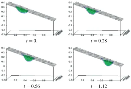
By observing the simulation results (Figure 4), it can be seen that the shape of droplet oscillates and the volume is preserved within the discretization error while the droplet moves. In addition, there are no particles moving out of the film during the motion. In other words, the number of particles representing the fluid is controlled well by the film during the motion. Judging from the obtained shapes of the droplet these results show a qualitative agreement with observations from the real experiments.

The above parameters were chosen so that they are close to the real values. However, a precise comparison with experimental data remains a future task.

t = 0 . t = 0 . 28

t = 0 . 56 t = 1 . 12

Figure 4: A droplet suspended under an inclined plane (simulation). Blue dots represent the film, green points represent the fluid inside the film and black dots represent the inclined plane.

4.2 Comparison with analytical result

Here we compute the stationary shape of a droplet with a given volume V using our coupled model and compare the result with the corresponding analytical solution. The analytical solution is given by the minimizer u of the functional

J ( u ) =

Ω

1

2 |∇u |

+ 1

2 ρ gu

χ

+ γ χ

dx .

Assuming radial symmetry u(x) = u(|x|) = u(r), it is possible to compute the minimizer analytically in the form

u ( r ) =

2 γ ρ g

I

(α √ ρ g ) I

(α √

ρ g )

1 − I

( r √ ρ g ) I

(α √

ρ g )

,

where α satisfies

α

α

√ ρ g 2

I

(α √ ρ g ) I

(α √

ρ g ) − 1

= V ρ g 2 π √

2 γ , and I

, I

are modified Bessel functions of the first kind.

For the parameters ρ = 1 , g = 9 . 8 ,γ = 0 . 5 , V = 0 . 00687 we obtain α = 0 . 2073.

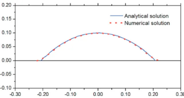
Figure 5: Cross-section of the analytical and numerical solutions.

The same parameters are used to calculate the steady-state solution by the coupled model. The initial condition is taken as a spherical cap with the volume V and the com- putations are continued until the change in the shape of the droplet is sufficiently small.

The cross-section of analytical and numerical solutions is plotted in Figure 5. The ob- tained radius of stationary droplet is α

= 0 . 2209 , which is slightly bigger than the analytical value. This is probably caused by the ε-smoothing of contact angle in our nu- merical model. Nevertheless, it is necessary to carry out detailed convergence analysis in order to fully validate the model.

5 Conclusions

We derive a simple model for the motion of a droplet moving on the plane. The film motion is a hyperbolic free boundary problem with volume-constraint, which was solved using the discrete Morse flow method. The fluid motion equations, on the other hand, were solved using the SPH method. Moreover, we showed a three-dimensional simula- tion of a droplet moving under an inclined plane. Comparison of numerical results with experimental data and analytical solution was performed.

Acknowledgement

The author expresses his gratitude to Professor Seiro Omata, for many ideas and advice

about the problem.

References

[1] E. GINDER, K. ˇSVADLENKA, A variational approach to a constrained hyperbolic free boundary problem,Nonlinear Analysis71, 2009, pp. e1527-e1537.

[2] K. HOSHINO, N. KIKUCHI,On a construction of weak solutions to linear hyperbolic partial differ- ential systems with the higher integrable gradients,J. Math. Sci.93, 1999, pp. 636-652.

[3] H. IMAI, K. KIKUCHI, K. NAKANE, S. OMATA, T. TACHIKAWA,A numerical approach to the asymptotic behavior of solutions of a one-dimensional hyperbolic free boundary problem,JJIAM18 (1), 2001, pp. 43-58.

[4] M. KAZAMA, S. OMATA, Modelling and computation of fluid-membrane interaction, Nonlinear Analysis71, 2009, pp. e1553-e1559.

[5] N. KIKUCHI,An approach to the construction of Morse flows for variational functionals,in ”Nematics - Mathematical and Physical Aspects”, ed.: J.-M. Coron, J.-M. Ghidaglia, F. H´elein, NATO Adv. Sci.

Inst. Ser. C: Math. Phys. Sci.332, Kluwer Acad. Publ., Dodrecht-Boston-London, 1991, pp. 775-786.

[6] K. KIKUCHI, S. OMATA,A free boundary problem for a one dimensional hyperbolic equation,Adv.

Math. Sci. Appl.9(2), 1999, pp. 775-786.

[7] G.R. LIU, M.B. LIU, Smooth Particle Hydrodynamics a Meshfree Particle Method,World Scientific Publishing, London, 2003.

[8] J.J. MONAGHAN, Simulating free surface flows with SPH,Journal of Computational physics110, 1994, pp. 399-406.

[9] S. OMATA,A numerical method based on the discrete Morse semiflow related to parabolic and hyper- bolic equation,Nonlinear Analysis30(4), 2003, pp. 2181-2187.

[10] S. OMATA, M. KAZAMA, H. NAKAGAWA, Variational approach to evolutionary free boundary problems,Nonlinear Analysis71, 2009, pp. e1547-e1552.

[11] K. ˇSVADLENKA, Mathematical analysis and numerical computation of volume-constrained evolu- tionary problems, involving free boundaries, PhD. thesis, Kanazawa University, Japan, 2008.

[12] K. ˇSVADLENKA, A new numerical model for propagation of tsunami waves,Kybernetika43(6), 2007, pp. 893-902.

[13] K. ˇSVADLENKA, S. OMATA,Construction of solutions to heat-type problems with volume constraint via the discrete Morse flow,Funks. Ekvac.50, 2007, pp. 261-285.

[14] T. YAMAZAKI, S. OMATA, K. ˇSVADLENKA, K. OHARA, Construction of approximate solution to a hyperbolic free boundary problem with volume constraint and its numerical compution, Advances in Mathematical Sciences and Applications16, 2006, pp. 57-67.

[15] H. YOSHIUCHI, S. OMATA, K. ˇSVADLENKA, K. OHARANumerical solution of film vibration with obstacle, Advances in Mathematical Sciences and Applications16, 2006, pp. 33-43.

[16] T. YOUNG, An essay on the cohesion of fluids, Philos. Trans. R. Soc. London95, 1805, pp. 65-87.