Change in house price structure with time and housing price index -Centered around the approach to the problem of structural change-

Change in house price structure with time and housing price index

-Centered around the approach to the problem of structural change- Chihiro SHIMIZU* Hideoki TAKATSUJI** Hiroya ONO** Kiyohiko G. NISHIMURA***

Abstract

The purpose of this study is to estimate the hedonic price index of secondhand condominiums while taking into account seasonal sample selection bias and structural changes, using the 23 wards of Tokyo as a subject. When housing price indices are estimated using a hedonic price model, the problem of temporal sample selection bias in addition to changes in the housing market structure should be considered. We propose an overlapping-period hedonic model (OPHM: this model was proposed by Ono, et al first), which can accommodate seasonal sample selection bias and structural changes. In addition, we estimate housing price indices for the 23 wards of Tokyo from 1986 through 2006, and demonstrate biases in price indices because of differences in the functions used in the models. Results of the estimation using the OPHM demonstrate that the structure of the housing market changes with time, and these changes occur continuously with time. It is also demonstrated that structurally restricted indices that do not account for structural changes involve a large time lag compared with indices that do account for structural changes during periods with significant price fluctuations. This study proposes a method of estimating hedonic housing price indices under the conditions of successively added data and structural changes.

Key Words: Hedonic housing price index, seasonal sample selection bias, (un)restricted hedonic model, overlapping-period hedonic model

JEL Code: C43 - Index Numbers and Aggregation, R31 - Housing Supply and Markets.

===================================

* Visiting Associate Professor, Center for Spatial Information Science (CSIS), University of Tokyo Associate Professor, The International School of Economics and Business Administration, Reitaku University

2-1-1 Hikarigaoka, Kashiwa-Shi, Chiba, 277-8686 Japan Tel. +81-(0)4-7173-3439, Fax. +81-(0)4-7173-1100 e-mail: cshimizu@reitaku-u.ac.jp

** Professor , The International School of Economics and Business Administration, Reitaku University 2-1-1 Hikarigaoka, Kashiwa-Shi, Chiba, 277-8686 Japan

***Member of the Policy Board, Bank of Japan

2-2-1 Hongoku-cho, Chuo-Ku, Tokyo 103-8660, Japan

1.Objectives of the study

The specifications and facilities of each house are different from each other in varying degrees, so there are no two houses of identical quality. Even when the specifications and facilities are identical, if the age of the building differs, the degree of deterioration differs accordingly, so that the houses are not identical.

In other words, houses have “particularity with few equivalents”. In addition to such a problem, the quality of houses (in particular, condominiums) changes with time owing to fairly rapid technological progress. Such characteristics are particularly evident in the housing market of Japan compared with the United States and other countries (Shimizu, Nishimura and Asami, 2004).

There are two approaches in constructing a housing price index that takes into account issues resulting from the above particularity with few equivalents and changes in quality: they are hedonic price model and the repeat-sales method. In the current study, we use hedonic price model to estimate the price indices of the secondhand condominium market in the 23 wards of Tokyo.

When the repeat-sales method and hedonic price model are compared, the following problems are noted for the respective methods.

In the repeat-sales method, the following two problems are noted: (i) a sample selection bias issue, that is, houses that are repeatedly on sale have different characteristics from the houses traded in the market (so-called lemons) (Clapp and Giaccotto, 1992), and (ii) accommodating qualitative changes and structural changes because of the assumption that there are no changes in the property characteristics and their parameters during the transaction period in the repeat-sales method (Case and Shiller, 1987, 1989;

Clapp and Giaccotto, 1992, 1998, 1999; Goodman and Thibodeau, 1998; Case, Pollakowski and Wachter, 1991).

Furthermore, the estimation of housing price indices by hedonic price model has the following two

major problems: (iii) the occurrence of bias in housing price indices because of the difficulty in

collecting all the variables required for the estimation of functions as well as because of the presence of

unobservable factors such as environmental variables (see Case and Quigley, 1991; Clapp, 2003), and

(iv) a structural change issue, that is, it is necessary to accommodate changes in the house price structure,

because the housing market is examined over a long period of time (Case, Pollakowski and Wachter, 1991; Clapp, Giaccotto and Tirtiroglu, 1991; Clapp and Giaccotto, 1992, 1998; Shimizu and Nishimura, 2006,2007). However, while the two approaches have problems in terms of estimation, it can also be shown that as the analysis period increases, the difference between the hedonic price index and the price index evaluated by the repeat-sales method decreases (Clapp and Giaccotto, 1998, 1999).

With regard to problem (i) of the repeat-sales method, because not all the transaction data are collected and estimated, the problem of sample selection bias also exists for hedonic price model , although its level is relatively low. Problems (ii) and (iv) occur in both the repeat-sales method and hedonic price model when housing price indices over a long period of time are estimated (i.e., there is a problem of coping with structural changes).

Regarding problem (iii), problems relating to the control of unobservable environmental variables can be avoided in the repeat-sales method (Case and Quigley, 1991; Case and Shiller, 1987, 1989; Thibodeau, 1997). Furthermore, the calculation procedure is simpler, and hence the calculation load is smaller in the repeat-sales method than in hedonic price model . Therefore, it has been considered that, at a glance, the repeat-sales method is more practical (Bourassa, Hoesli and Sun, 2006).

However, because the fluidity of housing markets is considerably lower (i.e., the market is thinner) in Japan than in the United States and other countries, and because institutional restrictions strongly suppress reselling within a short period, in accordance with the law based on the National Land Use Plan, problems with repeat-sales sample selection bias unique to Japan will still occur. If the repeat-sales method is to be applied in Japan, such a sample selection bias will be an extremely large problem, and in addition to that, the estimation of housing prices with high renewal frequency is impossible because of the small number of samples, and the estimation of indices in a limited area is difficult; consequently, the repeat-sales method is not a very practical method.

Under such circumstances, the importance of estimating hedonic housing price indices with high accuracy while solving the above problems involved in hedonic price model is extremely high in Japan.

Therefore, in this study, we focus on the greatest problem involved in hedonic price model, which relates

to changes in the market structure. Problem (iii) will be discussed in another report (according to Clapp (2003), unobservable variables are handled by adding coordinate data).

We start with the estimation of a structurally restricted hedonic model (hereafter, also referred to as the RHM) under the assumption of no changes in the market structure and a structurally unrestricted hedonic model (hereafter, also referred to as the URHM) under the assumption that the structure changes in each period (Case, Pollakowski and Wachter, 1991; Clapp, Giaccotto and Tirtiroglu, 1991).

In Section 2, the structures of the structurally restricted hedonic housing price index (hereafter, also referred to as the RHI) estimated using the restricted hedonic model and of the structurally unrestricted hedonic housing price index (hereafter, also referred to as the URHI) estimated using the unrestricted hedonic model are explained together with the repeat-sales index. This is aimed at clarifying the characteristics of hedonic price model in terms of estimation, by means of comparison with the repeat- sales method. Then, we propose a new housing price index taking into account structural changes and seasonal sample selection bias; the overlapping-period hedonic housing index (hereafter, also referred to as the OPHI). Data are explained in Section 3, and RHI, URHI and OPHI are estimated for the secondhand condominium market in the 23 wards of Tokyo, and the estimated housing price indices are evaluated in Section 4.

The results show temporal changes in the house price structure in the secondhand condominium market,

and in particular, regarding the floor space, the sign is reversed during some periods. Therefore, it is

necessary to estimate the price index taking into account structural changes. In addition, because housing

transactions in Japan tend to be concentrated in periods when large numbers of people move, the number

of samples varies considerably with the season; accordingly, seasonal sample selection bias should be

considered. To accommodate changes in the market structure and the problem of seasonal sample

selection bias, it has been demonstrated that OPHM with an overlapped estimate period τ of 12 months

is effective.

2.Changes in market structure and housing price indices

2.1.Structurally restricted hedonic housing price index (RHI) and structurally unrestricted hedonic housing price index (URHI)

Regarding the estimation of quality-adjusted housing price indices, the hedonic estimation method and the repeat-sales estimation method can be used. The price indices of the hedonic estimation method include the structurally restricted price index and the structurally unrestricted price index. We summarize these estimation methods, and clarify the characteristics of the hedonic price indices in terms of estimation in comparison with the repeat-sales method.

2.1.1.Structurally restricted hedonic housing price index: RHI

Assume that we have data for the house price and residential property characteristics, which are pooled for all the periods t = 1, 2, …, T, and that the number of data samples in each period is n

. A house price estimation model that can be used to obtain a structurally restricted price index is given as follows.

it s

s s ikt

K k

k

it

X D

P = ∑ β + ∑

δ + ε

=

=1 1

ln (1)

t = 1, 2, …, T.

i = 1, 2, …, nt

(designates ith data among the n

data samples in period t).

Pit

= price of house i in period t (designates ith data among the data in period t, instead of designating the same house i over each of the t periods).

β

= parameter of residential property characteristic k.

Xikt

= value of property characteristic k of house i in period t.

δ

= parameter of the time dummy variable in period s.

Ds

: when s = 1, this takes a constant value of 1 (constant term). When 2 ≤ s ≤ T, this is a time dummy variable, and it takes a value of 1 when s = t and a value of 0 otherwise.

ε

= random disturbance term.

This model is called the structurally restricted hedonic model (RHM) because it assumes that the

regression coefficient β

of the house-price determining factor X

is constant throughout all the periods.

From this, the RHI is obtained as follows. The estimated price P ˆ

of a house with residential property characteristic values {X

} (k = 1, 2, …, K) in period t (t = 1, 2, …, T) is given as follows.

t k

K k

k

t

X

P ^ˆ β ^ˆ δ ^ˆ δ ^ˆ ln

1

+ +

= ∑

=

(2)

1 1

1

ˆ ˆ

ln ˆ = ∑ β + δ

= k

K k

k

X P

(3)

Here, β ^ˆ

, δ ˆ

, δ ^ˆ

are estimated values of the parameters. Accordingly, the housing price index P ˆ

/ P ˆ

in period t, where the house price in period t = 1 is used as the reference, is obtained as follows.

t t

P P ˆ / ˆ ) δ ^ˆ

ln(

= (4)

In addition, the change in the price index from period t−1 to period t can be expressed as follows.

1

1

) ˆ ˆ

/ ˆ

ln( P ˆ

P

= δ

− δ

₍₅₎

In this case, the price index is obtained under the assumption of specific residential property characteristic values {X

}; however, as we can see in the above process, price indices are expressed using only time dummy variables without involving residential property characteristic values in the RHI.

2.1.2.Structurally unrestricted hedonic housing price index: URHI

Using similar data to those described above, a house price estimation model that can be used to obtain a

URHI is given as follows.

it t ikt K

k kt

it

X

P = ∑ β + δ + ε

=1

ln

(6)

Here, no time dummy variables are used, and instead, the parameter β

and a constant term δ

related to residential property characteristics are assumed to change in each period. Namely, because the model does not assume the restriction of constant parameters, it is called the URHM. From equation (6), the URHI is obtained as follows. The estimated price P ˆ

of a house with residential property characteristic values {X

} (k = 1, 2, …, K) in period t (t = 1, 2, …, T) is given as follows.

t k K k

kt

t

X

P ^ˆ β ^ˆ δ ^ˆ ln

1

+

= ∑

=

(7)

1 1

1

1

ˆ ˆ

ln ˆ = ∑ β + δ

= k

K k

k

X P

(8)

Therefore, the housing price index P ˆ

/ P ˆ

in period t, where the house price in period t = 1 is used as the reference, is obtained as follows.

ˆ ) ( ˆ ˆ )

( ˆ ˆ )

ˆ /

ln(

1

1

1

= ∑ β − β + δ − δ

= k t

K k

k kt

t

P X

P

(9)

In addition, the change in the price index from period t−1 to period t can be expressed as follows.

ˆ ) ( ˆ ˆ )

( ˆ ˆ )

ˆ /

ln(

1

1 ,

1 −

= −

−

= ∑

−

+

−

k

t k kt t

t

P X

P β β δ δ

(10)

Thus, for the URHI, price indices are obtained for specific residential property characteristics. When

specific residential property characteristics change, the price index changes accordingly.

2.1.3. Repeat-sales housing price index

Next, the repeat-sales method is summarized. For house h, it is assumed that its price is determined by the residential property characteristics and the time point of the transaction. It is also assumed that the residential property characteristics do not change with time, and the strength of their effect on price formation also does not change. Thus, the house price model in this case can be expressed as follows.

ht T

s s s hk

K k

k

ht

X D

P = ∑ β + ∑ δ + ε

=

=1 1

ln

(11)

Pht

is the price of house h in period t. Here, we assume that house h appears repeatedly in different periods.

is the value of property characteristic k of house h, which does not change with time.

Accordingly, we assume that parameter β

of X

also does not change with time. D

variable and equals 1 when s = t (the period of the transaction) and 0 otherwise. Here, we assume that D

= 1 (a constant term). δ

is the parameter of the time dummy variable. It is assumed that house h is subject to a transaction twice, in periods t

and t

, during the estimation period of t = 1, 2, …, T. The house prices in the periods of transaction can be expressed, using the above model, as follows.

1 1

1 1

1

ln

K k

k

ht

X

P = ∑ β + δ + δ + ε

=

(12)

2 2

2 1

1

ln

k k

ht

X

P = ∑ β + δ + δ + ε

=

(13)

From equations (12) and (13), the price change

1 2

/

ht

P

P is given as follows.

(

)

1 2 1

2

/ )

ln( P

P

= δ

− δ

+ ε

− ε

(14)

Therefore, in this model, the price change is determined from the difference in the two time points of the

transactions irrespective of residential property characteristics. We now formulate the model to estimate changes in the house price with respect to data collected for various transactions of houses at various time points. We obtain:

h T

s s s ht

ht

P D

P = ∑ δ + μ

=1

) /

ln(

, (15)

where μ

is a random disturbance term and D

second transaction (t = t

),

), and 0 in other periods. In addition, parameter δ

of each time dummy variable estimated using this model represents the price index of each period. This represents the typical repeat-sales model.

On the basis of the above summary of the indices and under the assumption that the market structure changes, the structurally restricted hedonic price index is problematic in that it has the restriction that parameters for X

are identical throughout all the periods. In the repeat-sales method, the same assumption that parameters for X

remain constant is adopted, and in addition, the very strong assumption that there are no changes in the property characteristics during the transaction period is adopted as well. The latter assumption is too strong for Japan. In practice, the values of houses change because of the extension and reconstruction, or renovation of buildings, and because of the development of physical damage accompanying the increasing age of buildings. In Japan, large-scale renovation is performed every couple of years, and the life of houses is short compared with that in Europe and the United States; therefore, house prices significantly decrease as the age of buildings increases. Moreover, because of the weak restrictions on city planning in Japan, it is extremely unrealistic to assume that there are no changes in the city environment or in building property characteristics.

In the URHM , although the restriction on parameters for X

can be eliminated, an assumption that the

parameters including error terms are independent in each period is necessary. However, in a real market,

it cannot be expected that the structure always changes randomly. In addition, a new issue arises. When

seasonal sample selection bias occurs. For example, in Japan there are periods with a large number of transactions, from January to March when many people move, and periods with a small number of transactions, such as July and August, and these seasonal changes in the number of transactions may affect and bias the price index. Thus, although the URHM can possibly accommodate structural changes, it disconnects the estimation from the continuity of the market conditions and generates the problem of seasonal sample selection bias.

2.2.Overlapping-period hedonic housing price index: OPHI

The URHI assumes that the market structure changes successively. Such a structural change of the market occurs as a result of various external shocks; it is considered that there is, in reality, a certain adjustment period before such a change penetrates into the market. Accordingly, regression coefficients should be regarded as changing successively rather than instantaneously. However, generally, the estimation of a model with structural changes is performed by dividing observation data into several periods with break points, then using the divided data of each period (for example, Ono et al,2004;

Shimizu and Nishimura, 2006; Shimizu and Nishimura, 2007). Namely, the continuity of the observation data is disconnected at the break points. Therefore, it is rather difficult to use such an estimation method, under the assumption of the occurrence of successive structural changes, to determine regression coefficients allowing for successive changes. Instead, it may be more natural and desirable to estimate regression coefficients on the basis of a process of successive change by taking a certain period length τ as the estimation period, and by shifting this period, similar to the process of obtaining moving averages.

This process can be formulated as follows.

Assuming that we have pooled data over the periods 1, 2, …T. With respect to some of these periods, i.e., a period length τ , we assume the following basic model.

it s

s s ikt

K k

k

it

X D

P = ∑ β + ∑

δ + ε

=

=1 1

ln

, (16)

where t = 1, 2, …, τ (taking part of the entire pooled data consisting of 1, 2, …T periods, namely, taking a certain period length τ , the periods within this range are numbered from 1 to τ ).

i = 1, 2, …, nt

(ith datum among n

items of data in period t).

Pit

: price of house i in period t.

β

: parameter of residential property characteristic k; β

is assumed not to change within the period length τ.

Xkit

: value of property characteristic k of house i in period t.

δ

: parameter of the time dummy variable in period s.

Ds

: when s = 1, this takes a constant value of 1 (constant term). When 2 ≤ s

dummy variable and takes a value of 1 when s = t and a value of 0 otherwise.

ε

: random disturbance term.

In addition, we express a period with length τ starting from period r among periods 1, 2, …T, as [r, r + τ

− 1]. Then, our estimation method is obtained by applying the above basic model to periods [1, τ], [2, τ

+ 1], …, [r,

+ τ

τ + 1, T] successively. From this, successive changes of the market structure can be reflected in changes in the parameters. We call this model the OPHM, and the period length τ , the overlapped estimate period length.

OPHM is a RHM with respect to a certain period length τ . Accordingly, the parameter of the time dummy variable represents the price index of each period with the starting period of length τ as the reference.

Thus, price indices can be obtained directly from the basic model within the period length τ . With the OPHM, models for all the periods are estimated by successively shifting the period length τ by one period. Here, the problem remains of how to connect the price indices obtained by the estimation in each period length τ to construct the price index for all periods. Our method is as follows.

We designate the housing price index throughout all the periods as q

. This represents the price index of period r among periods 1, 2, …T. We designate the reference period as period 1, and assume that q

= 0.

We also designate a parameter of the time dummy variable obtained by applying the basic model to the

data for the period length τ starting from period r among periods 1, 2, …T, i.e., [r,

τ

) ( ) ( 2 ) (

1

, ˆ , , ˆ

ˆ

δ

δ

δ _L by explicitly expressing the period r.

The procedure to obtain the housing price index q

is as follows.

(Set 1)

The basic model is applied to the first [1, τ ] period to obtain the parameter of the time dummy variable.

) 1 ( ) 1 ( 2 ) 1 (

1

, ˆ , , ˆ

ˆ δ δ

δ _L

Using these parameters, we define the price index q

(r = 1, 2, …, τ ) for the [1, τ ] period as follows.

1

= 0 q

) 1 2( 2

= δ ˆ q

) 1 3( 3

= δ ˆ

q ₍₁₇₎

･･･

) 1

ˆ

= δ q

(Set 2)

To obtain the next price index q

under the assumption that those up to q

have been determined as described above, an estimated amount, which is considered to be the change from q

to q

, is added to

. We consider that this estimated amount is based on the following parameters:

) 2 ( ) 2 2( ) 2

1(

, ˆ , , ˆ

ˆ δ δ

δ _{L , (18)}

which are determined by the estimation using the basic model for the next [2, τ + 1] period, as follows.

) 2 ( 1 ) 2 (

−

τ

δ

δ ₍₁₉₎

Accordingly, q

is defined as follows.

) (

1 −

+

=

+

−

τ

q δ δ

q ₍₂₀₎

(Set 3)

Similarly, to obtain the next price index q

under the assumption that those up to q

have been determined, an estimated amount, which is considered to be the change from q

to q

is added to

. Accordingly, on the basis of the parameters determined by the estimation of the basic model for the [r, τ + r − 1] period,

) ( ) ( 2 ) (

1

, ˆ , , ˆ

ˆ

δ

δ

δ _{L , (21)}

the estimated price index is defined as follows.

) (

2

1

q

q

=

+ δ

− δ

₍₂₂₎

Thus, we can obtain the price indices by OPHM for all periods.

Here, we note one point regarding the estimation of the basic model (equation (16)). With respect to the random disturbance term ε

, when we assume:

)

(

Var ε = σ _{, (23)}

it has been confirmed by our previous analysis that:

2

2 j

i

σ

σ ≠

( i ≠ j ) (24)

holds. Namely, heterogeneity of the variance is observed. Therefore, the basic model (equation (16)) is reestimated using feasible generalized least squares (FGLS). That is, σ ˆ

is obtained from the residual upon estimation using the basic model (equation (16)), and then the parameter is estimated using the following.

ˆ ) / ( ˆ ) / ( ˆ )

/ ˆ (

/ ) (ln

1 1

t it s

t s s t

ikt K

k k t

it

X D

P σ = ∑ β σ + ∑

δ σ + ε σ

=

=

(25)

2.3.Setup of estimation model

In this study, the secondhand condominium market in the 23 wards of Tokyo is used as the analytical subject. The basic equation of the RHM is as follows.

∑ ε

∑

∑

∑

∑

+ +

+

+ +

+

=

l

l l k

k k

j

j j i

i i h

h h

TD a RD

a

LD a Z

a X

a a

FS RP

・

・

・

5 4

3 2

1

0

log log

/ log

(26)

RP: Resale price of condominium (yen) Xh

: Main variables

FS: Floor space (square meters) Age: Age of building (months)

TS: Time to the nearest station (minutes) TT: Travel time to central business district Zi

: Other variables

BS: Balcony space (square meters) NU: Number of units

BC: Other building characteristics

RT: Market reservation time (weeks) LDj

: Location (ward) dummy (j = 0 … J)

: Railway line dummy (k = 0 … J)

: Time dummy (l = 0 … K)

Residential property characteristics as explanatory variables include floor space (FS), time to nearest station (TS), travel time (TT) to the central business district (CBD), age of building (Age), area of balcony (BS) and other building property characteristics (Z

), as well as a railway dummy variable (RD

) and location (ward) dummy variable (LD

) as location factors. In addition, we have a time dummy variable (TD

). The regression coefficient of this time dummy variable (a

) represents the secondhand condominium price index. In the RHM, the estimation is performed using this equation with pooled data in the periods t = 1 ··· T.

In contrast, the basic equation of the URHM is given by equation (27) below; this is the equation of the RHM from which the time dummy variable is excluded. Estimation is performed for each period using the data of that period (period t). Setting the period length to one month, a model is estimated for all periods. Then, using the estimated models and the assumption of houses having the same quality, the price of the houses in each period is estimated and its change-over time is examined.

∑ + ε

∑ +

∑ +

∑ + +

=

k tk tk

j j j

i ti ti

h th th

t

t

FS a a X a Z a LD a RD

RP /

log

log

・

・

log

T

t = 1 L L L (27)

Using the OPHM, the RHM of equation (26) is adopted for the estimation period length τ .

3.Data

3.1.Secondhand condominium price data

The subject of the analysis is the 23 wards of Tokyo metropolitan area (621 square kilometers), and the

analysis period is approximately 20 years between January 1986 and September 2006.

As the main information source, we used the prices of secondhand condominiums published in Residential Information Weekly (or Shukan Jyutaku Joho in Japanese) published by RECRUIT, Co. This magazine provides information on the quality and asking price of listed properties on a weekly basis, and includes the historical price data of individual properties from the time they are placed in the magazine for the first time until they are removed because of sale or other reasons. There are three items of information regarding the price: i) the initial asking price (first offer price) upon appearance in the market, ii) the price upon removal from the magazine (estimated purchase price: first bid price), and iii) the transaction price, which are collected as a sample. The first asking price represents the seller’s desired price rather than the market value. In contrast, some of the transaction prices may partly reflect the specific situations of individual transactions such as the desire for a quick sale or hasty purchase.

Therefore, among the information published in Residential Information Weekly, we decided to use the price when the listing of the house is removed from the magazine upon the conclusion of the contract as the explanatory variable in the model. The price at the time of removal from the magazine is the first bid price offered by a prospective buyer, such a bid is offered through the process in which several particulars of quality and price are disclosed to the market via the magazine, and the price is decreased until the buyer responds to that information. Thus, the price we used indicates the upper range of possible bid prices and can be regarded as a competitive market price that is relatively free from individual specific conditions associated with transactions.

3.2.Data regarding house quality

In the condominium market, while condominiums with light-gauge steel structures are also included, transactions are mainly for condominiums with reinforced concrete (RC) structures or steel-reinforced concrete (SRC) structures; therefore, we used condominiums with RC or SRC structures as the subject of our study. A list of data analyzed is shown in table 1.

The transport accessibility of each condominium location is represented by the TT to the CBD and the

TS. The former is measured in the following way. First, we defined the CBD. The Tokyo Metropolitan

area is composed of the 23 wards of Tokyo as its center, with a dense railway network developed therein.

We designated seven terminal stations, which include six on the Yamanote Line, Tokyo, Shinagawa, Shibuya, Shinjuku, Ikebukuro, and Ueno, as well as Otemachi as the central station of the Tokyo Metro (Teito Rapid Transit Authority). Then, we investigated average travel times during the day from each station to the seven terminal stations, and set the minimum value as the TT to the CBD for that station.

By considering travel times to multiple terminal stations, the timesaving effect of a new railway development on the whole transport network can be embedded into the model. When a new line is developed or a new station is constructed, or when a timetable is changed, this index will change.

Therefore, travel times are renewed once every half year (April and October).

Regarding TS, different means of transportation are available. There are three transportation means: on foot, by bus and by car. However, because a very dense transportation network is established in the 23 wards of Tokyo, and many condominiums are built in transportation-convenient areas, condominiums only within walking distance or bus-transportation distance are included in the analysis data. Therefore, any difference in the transportation distance between the former and latter is controlled for using the bus dummy variable (BD). In addition, the walking time (in minutes) is recorded when the condominium is within walking distance, and the walking time from the condominium to the bus stop and the on-board time from the bus stop to the nearest station (in minutes) are recorded in the case of condominiums in a bus-transportation area. The TS is defined as; (walking time to nearest station) + (walking time to the bus stop) + (on-board time from the bus stop to the nearest station). Then, with respect to the bus- transportation area, the cross term of the constant dummy variable with the TS is incorporated in the BD.

Details of the model are described below.

The sale price of each property is also affected by the fluidity and thickness of the market. The time

spent until the contract is concluded is considered to be affected by the period and location and by the

level of activity of transactions in the market. We explain such market factors using variables such as

market reservation time (RT). This is the time period between the date when a house is placed on the

market by a seller, and the time period when a buyer appears. Properties with a long RT are regarded as those having a price higher than the equilibrium price, or those in a thin market. Conversely, properties with a short RT are regarded as those in a market with high fluidity or those having a price close to or lower than the equilibrium price. For our purposes, the RT is defined as the time period from when the property is listed in the magazine for the first time until it is removed from the magazine.

We also identified some quantitative measures representing building property characteristics. They are

when the contract is concluded. NU is regarded as a proxy variable for the grade of the entire condominium and the quality of the common space. In addition, we created other dummy variables: the ground-floor dummy variable is used because the price of a ground-floor property is expected to be lower than that of higher-floor properties, and the highest-floor dummy variable is used because the price is expected to again be higher on the top floor. In terms of the direction of properties, such as whether their opening parts are south facing or not, we define a south-facing dummy variable (SD).

Furthermore, we define a ferroconcrete structure dummy variable (FD) to incorporate the difference in structural strength.

The above variables are all related to the location or building characteristics of condominiums. It is reasonable to assume that other regional factors may also affect the house price. Therefore, we set an administrative-area dummy variable, LD, to reflect differences in the quality of public services, as well as the “Ji-Gurai” or area rank. Furthermore, the railway dummy variable, RD, represents the price structure for condominiums along railway lines, because most Japanese residential developments have been carried out along railway lines.

Finally, the time dummy variable (TD) is used to control for differences in the prices between different

time periods.The observation data consist of 211,179 samples collected between January 1986 and

September 2006.

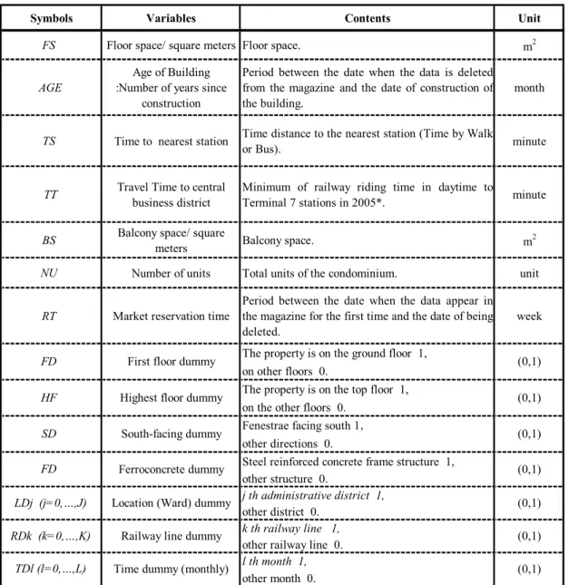
Table 1. List of analyzed data.

Symbols Variables Contents Unit

FS Floor space/ square meters Floor space. m²

AGE

Age of Building :Number of years since

construction

Period between the date when the data is deleted from the magazine and the date of construction of the building.

month

TS Time to nearest station Time distance to the nearest station (Time by Walk

or Bus). minute

TT Travel Time to central business district

Minimum of railway riding time in daytime to

Terminal 7 stations in 2005*. minute

BS Balcony space/ square

meters Balcony space. m²

NU Number of units Total units of the condominium. unit

RT Market reservation time

Period between the date when the data appear in the magazine for the first time and the date of being deleted.

week The property is on the ground floor 1,

on other floors 0.

The property is on the top floor 1, on the other floors 0.

Fenestrae facing south 1， other directions 0.

Steel reinforced concrete frame structure 1, other structure 0.

j th administrative district 1, other district 0.

k th railway line 1, other railway line 0.

l th month 1, other month 0.

TDl (l=0,…,L) Time dummy (monthly) (0,1)

*Terminal Staion : Tokyo,Shinagawa,Shibuya,Shinjuku,Ikebukuro,Ueno, and Ootemachi

LDj (j=0,…,J) Location (Ward) dummy (0,1)

RDk (k=0,…,K) Railway line dummy (0,1)

FD Ferroconcrete dummy (0,1)

HF Highest floor dummy (0,1)

SD South-facing dummy (0,1)

FD First floor dummy (0,1)

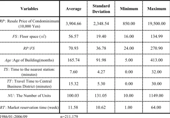
3.3.Statistical distribution of secondhand condominium price data

Table 2 shows descriptive statistics of the major variables. The average resale price of a condominium is 39.04 million yen, the minimum value is 8.50 million yen, and the maximum value is 195.00 million yen, with a fairly large standard deviation of 23.48 million yen. The data include a wide range of condominiums from studio-apartment-class small properties to the so-called 100-million-yen-class large properties. The average unit price is approximately 0.7 million yen/m

with a right-skewed distribution.

Regarding the FS, the minimum value is 16.00 m

, the maximum value is 134.99 m

, and the average is 56.57 m

, including all condominiums from single-person households to large-family condominiums.

Regarding the Age, the average value is 165 months (13.75 years), with a maximum value of 413 months (34.42 years). Because the history of condominiums in Japan is short, it is expected that this index will increase over time.

Regarding the TS, we only observed the distribution of data on the time axis; there are properties with a minimum value of 0 minutes that are located in front of a station. The maximum value is 32 minutes and the average value is 7.60 minutes. On average, while many properties are conveniently located, some are beyond walking distance. This indicates that, in general, convenience is emphasized in the construction of condominiums because of the required characteristics of condominiums.

Regarding the TT to the CBD, the average is 15 minutes with a maximum value of 30 minutes,

indicating that most condominiums are concentrated in areas of high convenience.

Table 2. Summary of statistical values of secondhand condominium price data.

Variables Average Standard

Deviation Minimum Maximum RP: Resale Price of Condominimum

(10,000 Yen) 3,904.66 2,348.54 850.00 19,500.00

FS: Floor space (㎡) 56.57 19.40 16.00 134.99

RP/FS 70.93 36.78 24.00 270.90

Age:Age of Building(months) 165.74 91.98 5.00 413.00

TS: Time to the nearest station:

(minutes) 7.60 4.27 0.00 32.00

TT: Travel Time to Central

Business District (minutes) 15.32 5.30 0.00 30.00

NU: The Number of Units 100.03 131.05 10.00 1149.00

RT: Market reservation time (week) 11.58 10.62 1.00 64.00

1986/01-2006/09 n=211,179

4.Estimation results

4.1.Estimation of RHI

The estimated RHI for the 23 wards of Tokyo is as follows.

+ ∑ + ∑

+ ∑

−

−

−

+

− +

−

× +

−

−

−

− +

+

−

−

− +

=

j j i i h

h LD RD TD

SD FD

HF FF

WT BD

BD

NU TT

TS Age

FS FS

RP

3 2

1

) 790 . 10 ( ) 150 . 10 ( ) 000 . 8 ( ) 210 . 19 ( )

970 . 6 ( ) 140 . 13 (

0093 . 0 097 . 0 018

. 0 026

. 0 ) log (

058 . 0 276

. 0

) 90 . 40 ( )

21 . 36 ( ) 69 . 99 ( ) 38 . 337 ( )

81 . 10 ( ) 23 . 498 (

log 019 . 0 log 117 . 0 log 078 . 0 log 189 . 0 log 0126 . 0 631 . 4 / log

β β

β 　

・

・

・

・

・

・

・

・

・

・

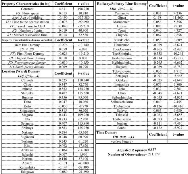
Adjusted R-square: 0.837 Number of observations: 211,178

Because the coefficient of determination adjusted for the degrees of freedom is 0.837, the estimated model has a fairly high explanatory power (refer to Table 3 for details).

Because the data was pooled for sales between 1986 and 2006, we corrected the time point by forcibly introducing the TD, so that the structure of the secondhand condominium price was estimated using property characteristics specific to condominiums and the RD. Among the property characteristics specific to condominiums, FS, BS and NU have positive values, and Age,

estimated with negative values.

First, regarding FS, the unit price was shown to increase with increasing floor space. A similar tendency was observed for BS and NU. This indicates that consumers show a strong preference for the floor space of each property as well as the floor space of the entire condominium.

As Age increases, we expect not only functional deterioration but also economic deterioration because of the improvement of facilities in newer condominiums. The results obtained showed that as TS and TT to the CBD increase, the convenience decreases because of the greater distance from populated areas, resulting in a decrease in the price.

Furthermore, the level of public service differs for each administrative ward, and there are broad

differences in the residential environment depending on administrative cities and wards or railway line

areas, which cannot be taken into consideration in our estimated function; therefore, these differences

were estimated using the dummy variables.

Table 3. Estimation results of the RHM: 23 wards of Tokyo.

Method of Estimation OLS

Dependent Variable

RP: Resale Price of Condominiums (in log) Independent Variables

Property Characteristics (in log) Coefficient t-value Railway/Subway Line Dummy

Constant 4.631 498.230 LDk (k=0,…,K)

FS: Floor space 0.013 10.810 Yamanote 0.033 4.236

Age: Age of building -0.190 -337.380 Ginza 0.158 11.460

TS: Time to the nearest station -0.078 -99.690 Marunouchi 0.056 5.556

TT: Travel Time to CBD -0.040 -36.210 Hibiya 0.085 9.039

NU: Number of units 0.019 40.900 Tozai 0.040 4.727

RT: Market reservation time 0.014 32.530 Chiyoda 0.067 7.858

Property Characteristics (dummy variables) Coefficient t-value ^{Yurakucho 0.053 3.609}

BD: Bus Dummy -0.276 -13.140 Hanzomon -0.029 -2.621

TS × BD 0.059 6.970 ToeiAsakusa -0.265 -2.420

FF: First Floor Dummy -0.026 -19.210 ToeiShinjuku -0.338 -10.244

HF:Highest floor dummy 0.018 8.000 Keihinkyukou -0.214 -15.225

FD:Ferroconcrete dummy -0.010 -10.150 Keihintohoku -0.265 -6.692

SD:South-facing dummy 0.009 10.790 Ikegami -0.089 -6.782

Location (Ward) Dummy Tokyutoyoko 0.036 1.712

LDj (j=0,…,J) Setagaya -0.091 -5.465

Chiyoda 0.625 110.740 Odakyu -0.025 -1.649

Chuo 0.347 82.770 Inogashira 0.076 5.800

minato 0.552 154.730 keio 0.032 2.361

Shinjuku 0.407 115.620 Chuo -0.045 -1.621

Bunkyo 0.356 95.060 Seibushinjuku -0.053 -4.024

Taito 0.047 10.080 Seibuikebukuro 0.040 2.455

Koto -0.030 -8.970 Toubutojou -0.126 -10.416

Shinagawa 0.315 86.020 Saikyo 0.065 5.680

Meguro 0.443 109.280 Takasaki -0.063 -5.655

Ota 0.233 62.930 Toubuisezaki -0.073 -2.694

Setagaya 0.407 115.890 Jouban -0.111 -7.410

Shibuya 0.583 155.950 Soubu -0.122 -5.927

Nakano 0.284 65.620 Time Dummy

Suginami 0.248 60.990 TDl (l=0,…,L)

Toshima 0.243 61.220 yes(see Figure)

Kita 0.092 17.620

Arakawa -0.064 -14.580 Adjusted R square=0.837

Itabashi 0.007 1.960 Number of Observations=211,179

Nerima 0.146 37.100

Adachi -0.171 -43.080

Katsushika -0.144 -38.390

Edogawa -0.080 -21.890

Coefficient t-value

Coefficient t-value

Coefficient t-value

4.2.Estimation of URHI

Next, we estimated the URHM. In accordance with the definition of equation (27), we divided the data into t periods (here, monthly) and estimated the structure of house prices. Regarding the price index, we estimated the prices of secondhand condominiums in each period by substituting the specific residential property characteristics common to all periods into the explanatory variables, and obtained the structurally unrestricted hedonic housing price indices relative to the reference period based on the estimated prices.

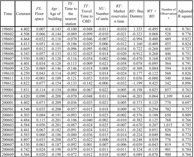
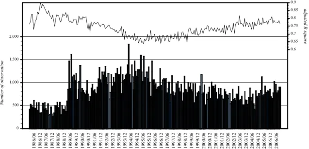
Table 4 shows the estimated regression coefficients of the major variables, and Fig. 1 shows changes in the number of samples and the coefficient of determination adjusted for the degrees of freedom.

The adjusted coefficient of determination decreased from 1986 through 1995, then increased from 1996.

However, on the whole, it maintained an average of around 0.75, showing fairly good results.

The number of samples was approximately 500 per month from 1986 through 1989, which then increased significantly to an average value of 844. However, there is more than a threefold difference depending on the month. In each year, transactions are concentrated from January to March, which is the end of the fiscal year, when there are large movements of people in Japan, and the number of transactions significantly decreases around July and August, thus showing seasonal changes. However, there is no apparent correlation between the number of samples and adjusted coefficient of determination.

Next, we focused on the regression coefficients of the estimated model. Table 5 shows descriptive statistical values for the regression coefficients over 250 periods. Figs 2–6 show changes in the regression coefficients with time. All of the regression coefficients show major fluctuations in each period or every several periods. However, the fluctuations show a certain tendency, although not a gradual change with time. In addition, we can see that all the variables are around (higher or lower than) the regression coefficients estimated using the RHM.

Using the data in Table 5, we calculated the coefficients of variance (standard deviation/average): FS =

2.428, Age = –0.179, TS = –0.232, TT to CBD = –0.779. In other words, FS shows the largest change,

including a change of the sign (+/–), followed by TT to the CBD, TS, and Age.

Table 4. Estimation results of the URHM : the 23 wards of Tokyo: 1986/01–2006/09.

Time Constant FS: Floor space

Age: Age of building

TS: Time to

the nearest station

TT: Travel Time to

CBD NU: Number of units

RT: Market reservatio

n time

BD: Bus Dummy

WT × BD

Number of Observation

s

Adjusted R square

198601 4.402 0.007 -0.143 -0.100 -0.048 -0.011 -0.010 1.333 -0.495 416 0.761 198602 4.508 0.066 -0.144 -0.089 -0.099 -0.010 -0.021 -0.323 0.068 528 0.776 198603 4.464 -0.032 -0.110 -0.070 -0.046 -0.007 -0.022 -0.994 0.480 489 0.823 198604 4.413 0.051 -0.161 -0.106 -0.029 0.006 -0.012 1.160 -0.489 455 0.824 198605 4.669 0.012 -0.155 -0.096 -0.095 -0.002 -0.034 0.722 -0.268 605 0.727 198606 4.343 0.057 -0.133 -0.132 -0.025 0.014 -0.020 -0.912 0.268 446 0.751 198607 3.930 0.083 -0.120 -0.116 -0.054 0.002 -0.046 -0.470 0.168 430 0.785 198608 4.401 0.034 -0.128 -0.113 -0.009 0.021 -0.058 0.078 -0.095 564 0.791 198609 4.526 0.069 -0.146 -0.146 -0.018 0.008 -0.020 -0.308 0.084 394 0.838 198610 4.250 0.043 -0.114 -0.092 -0.025 0.014 -0.024 0.177 -0.122 560 0.826 198611 4.310 -0.001 -0.109 -0.121 0.053 0.010 -0.031 0.036 -0.080 340 0.866 198612 4.822 0.077 -0.154 -0.133 -0.142 -0.006 -0.032 -1.199 0.425 342 0.896 199001 5.831 -0.114 -0.154 -0.084 -0.067 0.022 0.005 -0.198 0.025 857 0.763 199501 4.820 0.090 -0.208 -0.070 -0.048 0.011 0.044 -0.203 0.064 1,109 0.641 200001 4.402 0.071 -0.209 -0.036 -0.035 0.021 0.005 -0.373 0.125 778 0.697 200501 4.548 0.035 -0.208 -0.057 -0.015 0.018 0.009 -0.752 0.294 702 0.757 200601 4.303 0.084 -0.191 -0.093 -0.011 0.023 -0.002 -0.576 0.188 650 0.809 200602 4.484 0.115 -0.201 -0.106 -0.040 -0.002 -0.010 -0.382 0.125 768 0.766 200603 4.584 0.056 -0.201 -0.087 -0.024 0.025 -0.007 -0.670 0.207 1,015 0.785 200604 4.441 0.067 -0.182 -0.091 -0.024 0.012 -0.011 -0.242 0.051 826 0.775 200605 4.583 0.060 -0.186 -0.080 -0.036 0.015 -0.014 -0.224 0.049 966 0.774 200606 4.807 0.033 -0.208 -0.072 -0.022 0.000 -0.018 -0.248 0.039 776 0.775 200607 4.530 0.063 -0.187 -0.092 0.001 0.007 -0.006 -0.039 -0.043 819 0.770 200608 4.742 0.024 -0.198 -0.079 -0.015 0.011 -0.011 0.324 -0.135 901 0.784 200609 4.566 0.020 -0.198 -0.072 0.012 0.018 -0.005 0.089 -0.070 900 0.766

0 500 1,000 1,500 2,000

1986/06 1986/12 1987/06 1987/12 1988/06 1988/12 1989/06 1989/12 1990/06 1990/12 1991/06 1991/12 1992/06 1992/12 1993/06 1993/12 1994/06 1994/12 1995/06 1995/12 1996/06 1996/12 1997/06 1997/12 1998/06 1998/12 1999/06 1999/12 2000/06 2000/12 2001/06 2001/12 2002/06 2002/12 2003/06 2003/12 2004/06 2004/12 2005/06 2005/12 2006/06 0.6 0.65 0.7 0.75 0.8 0.85 0.9

Number of observation adjusted R square

Figure1.Estimation accuracy of the URHM: between 1986/01 and 2006/09.

Table 5. Statistical values of major regression coefficients (URHM).

Average Standard

deviation Skewness Kurtosis FS:Floor space/square

meters 0.013 0.033 0.081 -0.758 -0.627

Age:Age of building -0.190 -0.185 0.033 0.474 0.110

WT:Distance to

nearest station -0.078 -0.082 0.019 -0.640 0.799

TT:Travel Time to central business

district

-0.040 -0.041 0.032 -0.320 0.136

Adjusted-R Square 0.837 0.741 0.054 0.190 -0.379

Number of Samples 211,179 844.720 282.977 0.369 0.123

1986.01 - 2006.09:Monthly ,Number of Mode=250 NRHI:Summary statistics of estimated parameter Principal Independent

Variables

RHI:1986.01 - 2006.09

3.5 4 4.5 5 5.5 6 6.5

1986/06 1986/12 1987/06 1987/12 1988/06 1988/12 1989/06 1989/12 1990/06 1990/12 1991/06 1991/12 1992/06 1992/12 1993/06 1993/12 1994/06 1994/12 1995/06 1995/12 1996/06 1996/12 1997/06 1997/12 1998/06 1998/12 1999/06 1999/12 2000/06 2000/12 2001/06 2001/12 2002/06 2002/12 2003/06 2003/12 2004/06 2004/12 2005/06 2005/12 2006/06

NRHI Coefficient RHI

Fig2. Time profile of regression coefficient of the URHM, constant term cnst: 1986/01–

2006/09.

-0.2 -0.15 -0.1 -0.05 0 0.05 0.1 0.15 0.2

1986/06 1986/12 1987/06 1987/12 1988/06 1988/12 1989/06 1989/12 1990/06 1990/12 1991/06 1991/12 1992/06 1992/12 1993/06 1993/12 1994/06 1994/12 1995/06 1995/12 1996/06 1996/12 1997/06 1997/12 1998/06 1998/12 1999/06 1999/12 2000/06 2000/12 2001/06 2001/12 2002/06 2002/12 2003/06 2003/12 2004/06 2004/12 2005/06 2005/12 2006/06

NRHI

RHI

Coefficient

Fig3. Time profile of regression coefficient of the URHM, floor space FS: 1986/01–

2006/09.

-0.3 -0.25 -0.2 -0.15 -0.1 -0.05

1986/06 1986/12 1987/06 1987/12 1988/06 1988/12 1989/06 1989/12 1990/06 1990/12 1991/06 1991/12 1992/06 1992/12 1993/06 1993/12 1994/06 1994/12 1995/06 1995/12 1996/06 1996/12 1997/06 1997/12 1998/06 1998/12 1999/06 1999/12 2000/06 2000/12 2001/06 2001/12 2002/06 2002/12 2003/06 2003/12 2004/06 2004/12 2005/06 2005/12 2006/06

NRHI

RHI

Coefficient

Fig4. Time profile of regression coefficient of the URHM, age of building Age:

1986/01–2006/09.

-0.16 -0.14 -0.12 -0.1 -0.08 -0.06 -0.04 -0.02

1986/06 1986/12 1987/06 1987/12 1988/06 1988/12 1989/06 1989/12 1990/06 1990/12 1991/06 1991/12 1992/06 1992/12 1993/06 1993/12 1994/06 1994/12 1995/06 1995/12 1996/06 1996/12 1997/06 1997/12 1998/06 1998/12 1999/06 1999/12 2000/06 2000/12 2001/06 2001/12 2002/06 2002/12 2003/06 2003/12 2004/06 2004/12 2005/06 2005/12 2006/06

NRHI RHI

Coefficient

Fig5. Time profile of regression coefficient of the URHM, time to nearest station TS:

1986/01–2006/09.