and Materials
Engineering
Copyright © 2013 by JSME
Analysis of In-Plane Problems
for an Isotropic Elastic Medium with
Many Circular Elastic Inclusions
Mutsumi MIYAGAWA
∗∗, Takuo SUZUKI
∗∗, Takanobu TAMIYA
∗∗and
Jyo SHIMURA
∗∗∗∗∗Dept.of Creative Manufacturing Tokyo Metropolitan College of Industrial Technology. Arakawa Campus
8-17-1, Minami-senju, Arakawa-ku, Tokyo 116-0003, Japan E-mail: [email protected]
∗∗∗Tokyo National College of Technology
1220-2, Kunugida-machi, Hachioji-shi, Tokyo 193-0997, Japan
Abstract
This paper presents general solutions for problems involving many circular elastic in-clusions that are perfectly bonded to an elastic medium(matrix) of infinite extent under in-plane deformation. These many elastic inclusions may have different radii, central points and possess different elastic properties. The matrix is assumed to be subjected to arbitrary loading, for example, by uniform stresses at infinity. The solutions were obtained through iterations of the M¨obius transformation as series with an explicit gen-eral term involving the complex potential functions of the corresponding homogeneous problem. This procedure is referred to as heterogenization. Using these solutions, sev-eral numerical examples are presented graphically.
Key words : Elasticity, In-Plane Problem, Many Circular Elastic Inclusions, Uniform Stresses
1. Introduction
A number of studies have examined the problems associated with disturbances around a single circular inclusion under in-plane loading, such as loading due to uniform stresses or a concentrated force at an arbitrary point. Therefore, these problems have many applications in engineering fields. These inclusion problems have proved to be very useful for mechanical analysis.
These problems have been developed further in order to observe the interacting distur-bances for multiple circular inclusions. However, these techniques have been applied using different numerical analysis methods such as the finite element method (FEM) or the bound-ary element method (BEM). So, for example, if one engineer is an expert in FEM analysis of a model, while another engineer is not, their results will not be the same. General solutions of multi-inclusion problems for the in-plane situation using the theory of elasticity have not yet been produced. The governing equation for the anti-plane problem is a harmonic equation, but for the in-plane problem, it is a biharmonic equation. Thus, it is difficult to satisfy the continuity of stresses and displacement on the boundary.
The purpose of the present study is to apply the reflection principle of Moriguchi(1), Dun-ders(2)and Sendeckyj(3)who investigated a single hole or inclusion in the in-plane problems, and the techniques of Honein(4)and Hirashima(5)∼(7) to consider anti-plane multi-inclusion
problems. We obtained general solutions(8)(9)for up to two circular inclusions. Using these
techniques, we expanded these problems to cases involving many circular inclusions. To ana-lyze the problem of rigid inclusions or holes(10), we need only change the elastic modulus of the inclusion to∞ (Rigid inclusions) or to 0 (Holes). In the present study, these inclusions have arbitrary arrangements, elastic modulus and sizes inside the matrix. Using this explicit
*
*Received 29 Aug., 2013 (No. T2-2011-JAR-0206) Japanese Original : Trans. Jpn. Soc. Mech.
pp.980-992 (Received 15 Mar., 2011) Eng., Vol. 77, No. 778, A (2011), [DOI: 10.1299/jmmp.7.553]
general solution, we present several numerical examples under uniform stresses at infinity.
2. Fundamental Equation and General Solution
2.1. Formulation of elastostatics for in-plane problems
In this section, we review the fundamental formulation of in-plane elastostatics and present the notation used herein. We consider the complex region z= x + iy, where i is the imaginary unit (i= √−1), to be infinite. Under in-plane deformations, there exist displace-ments ux and uy and stresses σx, σy, and τxy, which are obtained in Cartesian coordinates
only.
The formulation used to find the stresses and displacements is satisfied by the complex potential functionsϕ(z) and ψ(z), which are also used in the techniques of Moriguchi(1).
ux− iuy= 1 2GM [ κMϕ(z) −{zϕ0(z)+ ψ0(z)}]. (1) −Py− iPx= ϕ(z) +{zϕ0(z)+ ψ0(z)}. (2)
where a prime indicates differentiation with respect to the complex variables z and κM as
follows: κM= { (3− νM)/(1 + νM) Plane Stress 3− 4νM Plane Strain (3)
where GMandνMare the shear modulus and Poisson’s ratio for the matrix, respectively. Px
and Pyindicate the resultant forces that act from right to left along an arbitrary course from point A to point B in the matrix.
Px= ∫B A ( σxdy − τxydx ) , Py= ∫B A ( τxydy − σydx ) . (4)
Hence, the stresses are obtained as follows:
σx= 2Re[ϕ0(z)]− Re[zϕ00(z)+ ψ00(z)], σy= 2Re[ϕ0(z)]+ Re[zϕ00(z)+ ψ00(z)], τxy= Im [ zϕ00(z)+ ψ00(z)], (5)
where Re[ ] and Im[ ] are the real and imaginary parts, respectively, of the complex func-tion in parentheses, and the overbar indicates complex conjugafunc-tion.
2.2. General solution in the presence of a single circular hole
We first investigated the problem in the presence of a single circular elastic inclusion disturbing the in-plane loading, which was given by the complex potential functions φ(z) andψ(z) in the matrix. We considered the heterogeneous problem of the jth elastic circular
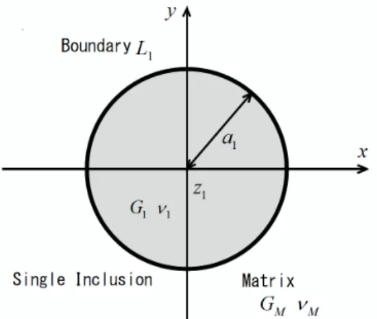
inclusion perfectly bonded to an elastic matrix of infinite extent. The matrix and the boundary produce an in-plane deformation, as shown in Fig. 1. We set the general boundary conditions of the tractions and displacements on the boundary Lj
(
i.e., z = zj+ ajeiθ
)
between the jth inclusion and the matrix, where ajand zj(= (0, 0)) are the radius and origin, respectively, of
the jthinclusion.
We will call the required continuity of the tractions and displacements the ”boundary conditions” along the circular interface.
Boundary conditions at Lj: P(M)x = P ( j) x , P (M) y = P( j)y , u(M)x = u ( j) x , u(M)y = u ( j) y . (6)
where, the upper subscripts (M) and ( j) mean the matrix and jthinclusion, respectively. In this
subsection, we use j= 1 because there is only one inclusion. The most general complexes for each region can be written as follows:
Fig. 1 Geometry of an infinite elastic medium with a single hole or rigid inclusion. Matrix: ϕM(z)= ϕ(z) + ˆf(z). (7) χM(z)= χm(z)+ ˆg(z). (8) jthinclusion: ϕIj(z)= ϕ(z) + h(z). (9) χIj(z)= χj(z)+ k(z). (10)
Based on Eqs.(1) and (2), we setχIj(z) in Eq.(10) as a first assistant function of the j
th inclu-sion. χIj(z)= zϕ 0 Ij(z)+ ψ 0 Ij(z). (11)
When the matrix is an isotropic material, using the mirror projection of a point that is produced by Moriguchi(1)on the boundary|z| = a
j, we setχM(z) in Eq.(8) as a first assistant function of
the matrix. χM(z)= a2j z ϕ 0 M(z)+ ψ0M(z). (12)
Also, we set χj(z) in Eq.(10) as a second assistant function of the jthinclusion.
χj(z)= γjzϕ0(z)+ ψ0(z). (13)
Eq.(11) is continuous with Eq.(12) on the boundary Lj. Therefore, we setχM(z) in Eq.(8) as a
second assistant function for the matrix in the following equation.
χm(z)= γj
a2
j
z ϕ
0(z)+ ψ0(z). (14)
where, γjis the unknown constant. Note that f, g, h, and k in Eqs. (7) ∼ (10) are determinate
functions, after we establish ˆf (z) and ˆg(z) in the following equations using the principle of mirror projection: ˆ f (z)= f(a2 j/z ) , g(z) = gˆ (a2 j/z ) . (15)
To satisfy the boundary conditions of Eq.(6) on the interface Lj, we continue the analysis of
the complex potential functionsϕ(z), χ(z) in the following equations. There is a detailed derivation in reference(9). Finally, we obtain the relations.
Matrix: ϕM(z)= ϕ(z) + αjχm(a2j/z). (16) χM(z)= χm(z)+ βjϕ(a2j/z). (17) jthinclusion: ϕIj(z)= ϕ(z) + βjϕ(z). (18) χIj(z)= χj(z)+ αjχj(z). (19)
Eqs. (16)∼(19) are obtained when the center of the jth inclusion coincides with the origin.
This problem is reduced to finding f, g, h, and k such that the continuities given by Eq. (6) are satisfied. Matrix: ϕM(z)= ϕ(z) + αjχm(Ajz). (20) χM(z)= χm(z)+ βjϕ(Ajz). (21) jthinclusion: ϕIj(z)= ϕ(z) + βjϕ(z). (22) χIj(z)= χj(z)+ αjχj(z). (23)
Where, αj, βjand γjare given as
αj= Gj− GM κMGj+ GM, β j= κMGj− κjGM Gj+ κjGM , γ j= 1+ βj 1+ αj. (24) κM= { (3− νM)/(1 + νM) Plane Stress 3− 4νM Plane Strain (25)
Gjandνjare the shear modulus and Poisson’s ratio for the jthinclusion, respectively. When
the jthinclusion is a rigid inclusion or hole, we only have to set G
jto a special value in the
following.
{α
j= 1/κM, βj= κM. Rigid inclusion (Gj→ ∞)
αj= −1, βj= −1. Hole (Gj→ 0)
(26)
In Eqs.(20)∼ (23), we consider the problem in the single circular inclusion ( j = 1) in the ma-trix. We have a strong conviction that these solutions coincide with the solution of Dunders(2) and Sendeckyj(3). The fundamental complex potential functionsφ(z) and ψ(z) are given by the
arbitrary loading described in a later section. To this end, we define Ajz=
a2j z− zj
+ zj, ( j = 1, 2). (27)
Moreover, Aj specifies the operator with respect to the complex variable z. Normally, the
left-hand side of Eq. (27) would be written as Aj(z). However, for convergence, in the present
paper we denote Ajz as in Eq. (27). Thus, AiAjz, for example, is expressed as follows:
AiAjz= Ai [ Aj(z) ] = a 2 i Aj(z)− zi + zi= a2 i a2 j z− zj + z j − zi + zi. (28)
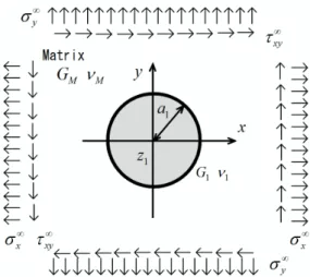
Fig. 2 Infinite elastic matrix with a single inclusion under uniform stresses.
2.3. Problem in the presence of a single circular inclusion under uniform stresses
In this section, we consider the problem of disturbing the uniform stressesσ∞x,σ∞y, and
τ∞
xyat infinity in Fig. 2. The fundamental complex potential functionsφ(z), ψ0(z) are given at
infinity|z| = ∞ as ϕ(z) = τ∗z, ψ0(z)= 2τ∗∗z. (29) where τ∗= σ∞x + σ∞y 4(1+ α1γ1) , τ∗∗= σ∞y − σ∞x 4 + i τ∞ xy 2 . (30)
These functions do not have a singularity inside the region aj < |z| < ∞ ( j = 1). We
next considered the functions obtained by substituting Eq. (29) into Eqs. (20) and (23), that coincide in the initial conditionsσ∞x,σ∞y, andτ∞xy at infinity. The second assistant function
χ1(z), defined in Eq. (13) at infinity|z| = ∞, reduces to
χ1(z)= γ1zφ0(z)+ ψ0(z). (31)
From Eq.(31), a second assistant functionχm(z) for the matrix is given as
χm(z)= γ1
a2 1
zφ
0(z)+ ψ0(z). (32)
The functions obtained by substituting Eq. (31) into Eqs. (20) and (23) are general solutions in this subsection, and we obtain the following:
Matrix: ϕM(z)= ( τ∗z+ α 1γ1τ∗ ) z+ 2α1τ∗∗A1(z). (33) χM(z)= 2τ∗∗z+ ( γ1τ∗+ β1τ∗ ) A1(z). (34) 1stinclusion: ϕI1(z)= (1 + β1)τ ∗z. (35) χI1(z)= (1 + β1)τ ∗z+ 2 (1 + α 1)τ∗∗z. (36)
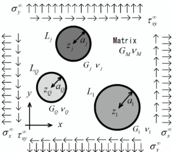
Fig. 3 Geometry of an infinite elastic matrix with many circular elastic inclusions.
2.4. General solution in the presence of many circular inclusions
In this section, we use the solution presented in the previous section as a starting point for obtaining the solution for many circular inclusions that have radii ajand origins zj( j= 1, 2, · · · , Q),
as shown in Fig. 3, where Gjandνjare the shear modulus and Poisson’s ratio for the jth
inclu-sion, respectively. To analyze the problem of rigid inclusions or holes, we need only change the coefficient Gj→ ∞ (Rigid inclusions) or to Gj→ 0 (Holes).
This matrix is given by the complex potential functionsφ(z) and ψ(z). We set the general boundary conditions given by Eq.(6), of the tractions and displacements. For the purpose of the multi-inclusion problem, we first considered the problem with three holes (i.e. Q = 3 ) as a simple case. After that, we produced the general solution for many holes (Q is arbitrary number). Using the same technique, we could satisfy the continuities given by Eqs. (1) and (2) for the boundary Lj. We first set the general functions ˆf1(z), ˆg1(z), h1(z) and k1(z) on L1
as follows: Matrix: ϕM(z)= ϕ(z) + ˆf1(z), (37) χM(z)= χm(z)+ ˆg1(z). (38) 1stInclusion: ϕI1(z)= ϕ(z) + h1(z), (39) χI1(z)= χ1(z)+ k1(z). (40) 2ndInclusion: ϕI2(z)= ϕ(z) + ˆf1(z), (41) χI2(z)= χ2(z)+ ˆg1(z). (42) 3rdInclusion: ϕI3(z)= ϕ(z) + ˆf1(z), (43) χI3(z)= χ3(z)+ ˆg1(z). (44)
These functions reduce to finding ˆf1(z), ˆg1(z), h1(z) and k1(z) such that the continuities on
L1are satisfied. The following equations are obtained using sets ˆf2(z), ˆg2(z), h2(z) and k2(z)
Matrix: ϕM(z)= ϕ(z) + α1χm(A1z)+ ˆf2(z), (45) χM(z)= χm(z)+ β1ϕ(A1z)+ ˆg2(z). (46) 1stInclusion: ϕI1(z)= ϕ(z) + β1ϕ(A1z)+ ˆf2(z), (47) χI1(z)= χ1(z)+ α1χ1(A1z)+ ˆg2(z). (48) 2ndInclusion: ϕI2(z)= ϕ(z) + α1χ2(A1z)+ h2(z), (49) χI2(z)= χ2(z)+ β1ϕ(A1z)+ k2(z). (50) 3rdInclusion: ϕI3(z)= ϕ(z) + α1χ3(A1z)+ ˆf2(z), (51) χI3(z)= χ3(z)+ β1ϕ(A1z)+ ˆg2(z). (52)
These functions reduce to finding ˆf2(z), ˆg2(z), h2(z) and k2(z) such that the continuities on
L2are satisfied. The following equations are obtained using sets ˆf3(z), ˆg3(z), h3(z) and k3(z)
on L3: Matrix: ϕM(z)= ϕ(z) + α1χm(A1z)+ α2χm(A2z)+ β1α2ϕ(A1A2z)+ ˆf3(z), (53) χM(z)= χm(z)+ β1ϕ(A1z)+ β2ϕ(A2z)+ α1β2χm(A1A2z)+ ˆg3(z). (54) 1stInclusion: ϕI1(z)= ϕ(z) + β1ϕ(A1z)+ α2χ1(A2z)+ β1α2ϕ(A1A2z)+ ˆf3(z), (55) χI1(z)= χ1(z)+ α1χ1(A1z)+ β2ϕ(A2z)+ α1β2χ1(A1A2z)+ ˆg3(z). (56) 2ndInclusion: ϕI2(z)= ϕ(z) + α1χ2(A1z)+ β2ϕ(z) + α1β2χ2(A1z)+ ˆf3(z), (57) χI2(z)= χ2(z)+ β1ϕ(A1z)+ α2χ2(A2z)+ β1α2ϕ(A1z)+ ˆg3(z). (58) 3ndInclusion: ϕI3(z)= ϕ(z) + α1χ3(A1z)+ α2χ3(A2z)+ β1α2ϕ(A1A2z)+ h3(z), (59) χI3(z)= χ3(z)+ β1ϕ(A1z)+ β2ϕ(A2z)+ α1β2χ3(A1A2z)+ k3(z). (60)
Applying the continuity on L3, we found ˆf3(z), ˆg3(z), h3(z) and k3(z). Note that the boundary
condition on L1is not satisfied for L2and L3 by the previous steps. For this reason, we may
set ˆf4(z), ˆg4(z), h4(z) and k4(z) to satisfy the continuity on L1.
Matrix: ϕM(z)= ϕ(z) + α1χm(A1z)+ α2χm(A2z)+ β1α2ϕ(A1A2z) + α3χm(A3z)+ β1α3ϕ(A1A3z)+ β2α3ϕ(A2A3z) + α1β2α3χm(A1A2A3z)+ ˆf4(z), (61) χM(z)= χm(z)+ β1ϕ(A1z)+ β2ϕ(A2z)+ α1β2χm(A1A2z) + β3ϕ(A3z)+ α1β3χm(A1A3z)+ α2β3χm(A2A3z) + β1α2β3ϕ(A1A2A3z)+ ˆg4(z). (62)
1stInclusion: ϕI1(z)= ϕ(z) + β1ϕ(A1z)+ α2χ1(A2z)+ β1α2ϕ(A1A2z) + α3χ1(A3z)+ β1α3ϕ(A1A3z)+ β2α3ϕ(A2A3z) + α1β2α3χ1(A1A2A3z)+ h4(z), (63) χI1(z)= χ1(z)+ α1χ1(A1z)+ β2ϕ(A2z)+ α1β2χ1(A1A2z) + β3ϕ(A3z)+ α1β3χ1(A1A3z)+ α2β3χ1(A2A3z) + β1α2β3ϕ(A1A2A3z)+ k4(z). (64) 2stInclusion: ϕI2(z)= ϕ(z) + α1χ2(A1z)+ β2ϕ(z) + α1β2χ2(A1z) + α3χ2(A3z)+ β1α3ϕ(A1A3z)+ β2α3ϕ(A2A3z) + α1β2α3χ2(A1A2A3z)+ ˆf4(z), (65) χI2(z)= χ2(z)+ β1ϕ(A1z)+ α2χ2(A2z)+ β1α2ϕ(A1z) + β3ϕ(A3z)+ α1β3χ2(A1A3z)+ α2β3χ2(A2A3z) + β1α2β3ϕ(A1A2A3z)+ ˆg4(z). (66) 3stInclusion: ϕI3(z)= ϕ(z) + α1χ3(A1z)+ α2χ3(A2z)+ β1α2ϕ(A1A2z) + β3ϕ(z) + α1β3χ3(A1z)+ α2β3χ3(A2z) + β1α2β3ϕ(A1A2z)+ ˆf4(z), (67) χI3(z)= χ3(z)+ β1ϕ(A1z)+ β2ϕ(A2z)+ α1β2χ3(A1A2z) + α3χ3(z)+ β1α3ϕ(A1z)+ β2α3ϕ(A2z) + α1β2α3χ3(A1A2z)+ ˆg4(z). (68)
We applied the continuity on L1, repeating the previous steps and obtaining these additional
terms each time. In this way, we could find the following explicit solution of the in-plane problem in the presence of many circular elastic inclusions. To this end, we used
Matrix: ϕM(z)= ϕ(z) + +∞∑ n=1 ωM∗ p(n)q(n)ϕ(M M p(n)q(n)z)+ +∞ ∑ n=0 αq(0)ωMp(n)∗q(n)χm(Aq(0)MM p(n)q(n)z), (69) χM(z)= χm(z)+ +∞∑ n=1 ωM∗∗ p(n)q(n)χm(MMp(n)q(n)z)+ +∞ ∑ n=0 βq(0)ωM∗∗ p(n)q(n)ϕ(Aq(0)MM p(n)q(n)z). (70) jthInclusion: ϕIj(z)= ( 1+ βj ) { ϕ(z) ++∞∑ n=1 ωj∗ p(n)q(n)ϕ(M j p(n)q(n)z)+ +∞ ∑ n=0 αq(0)ωj∗ p(n)q(n)χj(Aq(0)M j p(n)q(n)z) } ,(71) χIj(z)= ( 1+ αj ) { χj(z)+ +∞∑ n=1 ωj∗∗ p(n)q(n)χj(M j p(n)q(n)z)+ +∞∑ n=0 βq(0)ωj∗∗ p(n)q(n)ϕ(Aq(0)Mj p(n)q(n)z) } .(72)
The coefficients in the above expressions are given as follows. The arguments p(i), q(i)indicate
different arguments from the index i and p(i), q(i)have values from 1 to Q. In addition, δp(i)
q(i) is
Matrix: ωM∗ p(n)q(n)ϕ(M M p(n)q(n)z)= n ∏ i=1 Q ∑ p(i)=1 Q ∑ q(i)=1 {1 − (1 − δi 1)δ q(i−1) p(i) }(1 − δ p(i)
q(i))βp(i)αq(i)ϕ(Ap(i)Aq(i)z). (73)
αq(0)ωMp(n)∗q(n)χm(Aq(0)MM p(n)q(n)z)= δ n 0 Q ∑ q(0)=1 αq(0)χm(Aq(0)z) +(1 − δn 0) n ∏ i=1 Q ∑ q(0)=1 Q ∑ p(i)=1 Q ∑ q(i)=1 (1− δqp(i(i)−1))(1− δ p(i)
q(i))αq(0)βp(i)αq(i)χm(Aq(0)Ap(i)Aq(i)z).(74)
ωM∗∗ p(n)q(n)χm(MMp(n)q(n)z)= n ∏ i=1 Q ∑ p(i)=1 Q ∑ q(i)=1 {1 − (1 − δi 1)δ q(i−1) p(i) }(1 − δ p(i)
q(i))αp(i)βq(i)χm(Ap(i)Aq(i)z). (75)
βq(0)ωMp(n)∗∗q(n)ϕ(Aq(0)MM p(n)q(n)z)= δ n 0 Q ∑ q(0)=1 βq(0)ϕ(Aq(0)z) +(1 − δn 0) n ∏ i=1 Q ∑ q(0)=1 Q ∑ p(i)=1 Q ∑ q(i)=1 (1− δqp(i(i)−1))(1− δ p(i)
q(i))βq(0)αp(i)βq(i)ϕ(Aq(0)Ap(i)Aq(i)z). (76)
jthInclusion: ωj∗ p(n)q(n)ϕ(M j p(n)q(n)z)= n ∏ i=1 Q ∑ p(i)=1 Q ∑ q(i)=1 {1 − (1 − δi 1)δ q(i−1) p(i) }(1 − δ p(i) q(i))(1− δ q(i)
j )βp(i)αq(i)ϕ(Ap(i)Aq(i)z). (77)
αq(0)ωj∗ p(n)q(n)χj(Aq(0)Mj p(n)q(n)z)= δ n 0 Q ∑ q(0)=1 (1− δqj(0))αq(0)χj(Aq(0)z) +(1 − δn 0) n ∏ i=1 Q ∑ q(0)=1 Q ∑ p(i)=1 Q ∑ q(i)=1 (1− δqp(i(i)−1))(1− δ p(i) q(i))(1− δ q(i) j )
× αq(0)βp(i)αq(i)χj(Aq(0)Ap(i)Aq(i)z). (78)
ωj∗∗ p(n)q(n)χj(M j p(n)q(n)z)= n ∏ i=1 Q ∑ p(i)=1 Q ∑ q(i)=1 {1 − (1 − δi 1)δ q(i−1) p(i) }(1 − δ p(i) q(i))(1− δ q(i)
j )αp(i)βq(i)χj(Ap(i)Aq(i)z). (79)
βq(0)ωj∗∗ p(n)q(n)ϕ(Aq(0)M j p(n)q(n)z)= δ n 0 Q ∑ q(0)=1 (1− δqj(0))βq(0)ϕ(Aq(0)z) +(1 − δn 0) n ∏ i=1 Q ∑ q(0)=1 Q ∑ p(i)=1 Q ∑ q(i)=1 (1− δqp(i(i)−1))(1− δ p(i) q(i))(1− δ q(i) j )
× βq(0)αp(i)βq(i)ϕ(Aq(0)Ap(i)Aq(i)z). (80)
when we omit upper subscripts M and j from the above equation. Note that these functions have the following relations:
ϕ(Mp(n)q(n)z)= Q ∑ p(n)=1 Q ∑ q(n)=1 (1− δqp(n(n)−1))(1− δ p(n) q(n))ϕ(Mp(n−1)q(n−1)Ap(n)Aq(n)z). (81) χm(Aq(0)Mp(n)q(n)z)= Q ∑ p(n)=1 Q ∑ q(n)=1 (1− δqp(n(n)−1))(1− δ p(n) q(n))χm(Aq(0)Mp(n−1)q(n−1)Ap(n)Aq(n)z). (82)
we obtained the external theoretical solutions. After that, we show the analytic solutions in a concrete example.
2.5. General solution in the presence of many circular elastic inclusions under uniform stresses
Fig. 4 Infinite elastic medium with many elastic inclusions under uniform stresses.
In this section, we consider the problem in the presence of many circular elastic inclu-sions ( j = 1, 2, · · · , Q) disturbing the uniform stresses σ∞x, σ∞y andτ∞xy at infinity. The jth inclusions have the boundary Lj, origin zj, radius aj, shear modulus Gj, and Poisson’s ratio
νj, respectively, in Fig. 4.
where, τ∗ and τ∗∗ are known constants under the initial conditions that the uniform stressesσ∞x,σ∞y, andτ∞xyload at infinity|z| = ∞. These constants are given as
τ∗= σ∞x + σ∞y 4 Q + Q ∑ j=1 αjγj Q, τ∗∗=σ ∞ y − σ∞x 4 + i τ∞ xy 2 . (83)
After that, we consider the second assistant functionsχm(z), χj(z). At first, an arbitrary point
z has total Q mirror points as Ajz ( j= 1, 2, · · · , Q) on the circular boundaries Ljrespectively.
Then, the point z needs to coincide with the mirror points on Lj. From this, we set the mirror
point of the matrix as∑Qj=1ΓjAjz using the unknown valueΓj. Therefore, the second assistant
functionχm(z) of the matrix is given as
χm(z)= Q
∑
j=1
ΓjγjAjzφ0(z)+ ψ0(z) (84)
Next, we consider the second assistant function inside the jth inclusion. When, the arbitrary point z is inside the jthinclusion, the second assistant function of the jthinclusion is given as
χj(z)= γjzφ0(z)+ ψ0(z) (85)
These assistant functions are continuous on the boundary Lj. We obtained the Γj with the
following equation. Γj= 1 dj∆d−1 , dj= |z − zj| − aj, ∆d−1 = Q ∑ j=1 1 dj . (86)
In this problem, these functions do not have a singularity inside the region aj< |z| < ∞ ( j =
1, 2, · · · , Q). Therefore, the fundamental complex potential functions φ(z) and ψ0(z) are given at infinity|z| = ∞, as shown in Eq. (29). The functions obtained by substituting the above equation into Eqs. (69) and (70) are general solutions to this problem, and are obtained as follows: Matrix: ϕM(z)= τ∗z+ +∞∑ n=1 ωM∗ p(n)q(n)τ∗M M p(n)q(n)z ++∞∑ n=0 αq(0)ωMp(n)∗q(n) τ∗ Q ∑ j=1 ΓjγjAq(0)MMp(n)q(n)Ajz+ 2τ∗∗Aq(0)MM p(n)q(n)z ,(87) χM(z)= τ∗ Q ∑ j=1 ΓjγjAjz+ 2τ∗∗z+ +∞∑ n=1 ωM∗∗ p(n)q(n) τ∗∗ Q ∑ j=1 ΓjγjMMp(n)q(n)Ajz+ 2τ∗∗M M p(n)q(n)z ++∞∑ n=0 βq(0)ωM∗∗ p(n)q(n)τ∗Aq(0)MM p(n)q(n)z. (88) jthInclusion: ϕIj(z)= ( 1+ βj ) τ∗z++∞∑ n=1 ωj∗ p(n)q(n)τ∗M j p(n)q(n)z ++∞∑ n=0 αq(0)ωj∗ p(n)q(n) ( γjτ∗Aq(0)Mj p(n)q(n)z+ 2τ∗∗Aq(0)M j p(n)q(n)z ) ,(89) χIj(z)= ( 1+ αj ) γjτ∗z+ 2τ∗∗z+ +∞∑ n=1 ωj∗∗ p(n)q(n) ( γjτ∗M j p(n)q(n)z+ 2τ∗∗M j p(n)q(n)z ) ++∞∑ n=0 βq(0)ωj∗∗ p(n)q(n)τ∗Aq(0)M j p(n)q(n)z . (90)
These solutions coincide with the solution of Moriguchi(1) and Hirashima(5)(6) for reduction to the single-hole problem. The above coefficients are given by
Ap(n)Aq(n)z set = AInz+ BIn CI nz+ DIn . (n ≥ 1) AI n= a2q(n)− zq(n) 2 + zp(n)zq(n), BI n= (a2q(n)− |zq(n)| 2)z p(n)− (a2 p(n)− |zp(n)| 2)z q(n), CI n= zq(n)− zp(n), DIn= a2 q(n)− zq(n) 2 + zp(n)zq(n). (91) where we set Mp(n−1)q(n−1)zset= AII n−1z+ B II n−1 CII n−1z+ D II n−1 . (92)
We obtained the following relations from the above recursions. Mp(n)q(n)z= Mp(n−1)q(n−1)Ap(n)Aq(n)z set = AIInz+ BIIn CII nz+ DnII . (93) where, AII
n, BnII, CnIIand DIIn are expressed as the following recursions.
A0II= DII0 = 1, BII0 = CII0 = 0. AII n = (AnII−1A I n+ BnII−1C I n), BII n = (AnII−1B I n+ BnII−1D I n), CII n = (CIIn−1A I n+ DnII−1C I n), DII n = (CIIn−1B I n+ DnII−1D I n). (n ≥ 1) (94)
and Aq(0)z set = A III 0z+ B III 0 CIII 0z+ D III 0 , A0III= zq(0), BIII0 = a2 q(0)− |zq(0)|2, CIII 0 = 1, D III 0 = −zq(0). (95)
From the above relations, we obtained Aq(0)Mp(n)q(n)z= Aq(0)Mp(n−1)q(n−1)Ap(n)Aq(n)z set = AIVnz+ BnIV CIV n z+ DIVn . (96) where AnIV= A0IIIA II n+ B0IIIC II n, BnIV= A0IIIBIIn+ B0IIIDnII, CIV n = CIII0A II n + DIII0C II n, DIV n = CIII0B II n+ D0IIID II n. (n ≥ 1) (97) Subsequently, Ajz set = A V 0z+ B V 0 CV 0z+ D V 0 , AV0 = zj, BV0 = a2j− |zj|2, C0V = 1, DV0 = −zj. (98) and Aq(0)Mp(n)q(n)Ajz set = AVInz+ BVIn CVI nz+ DVIn , AVI n = AV0A IV n + CV0B IV n, BVIn = BV0A IV n + DV0B IV n, CVI n = AV0C IV n + C0VD IV n, DVIn = BV0C IV n + DV0D IV n. (n ≥ 1) (99) In addition, AI
n ∼ AVIn, BIn∼ BVIn, CIn∼ CnVI, DnI ∼ DVIn are complex constants using the index
n, which means the calculation of n-count, and they are known constants because they satisfy the above recursions. The signset= means that the sign makes a connection with the complex variables and complex coefficients on the right-hand side of the equation.
3. Numerical Examples
The fundamental series solutions derived in the preceding section are used here to analyze the following examples. We define the ratio of the shear modulus of the jth inclusion and
matrix ej= Gj/GM. If ejis greater than 1, the elasticity of the jthinclusion is harder than that
of the matrix; if ejis smaller than 1, it is softer than the matrix. We call ejthe elastic constant
ratio in this paper.
Then, we must account for the convergence of Eqs. (69)∼ (72). Generally, when adjoin-ing inclusions are near or tangential to each other, the relative error may be large; that is to say, the convergences of the series tend to be large. We use n with a tolerance of relative error within 1% under the n and n− 1 counts.
As an example, we produce the convergence properties of numerical examples in Fig.7. We consider a geometry having three circular inclusions with ej = 0.1 ( j = 1 ∼ 3) and
distance D/a1 = 0.1. In the plane stress problem, we denote the convergence properties of
the problem under the uniform stressσ∞y. Table1 shows the relative error [RE] of stresses and displacements on the boundary as the value of n changes, and Fig.5 is given by the Table1. From this figure, we can obtain a very precise value when we set n at a higher level. In this example, we set n that [RE] is lower than 1% using n= 9. Specifically, the tolerable value is confirmed to be sufficiently satisfied when we perform a general analysis using n = 10.
Table 1 Table of the relative errors [RE] uxandσθatθ = 0 in the calculation of the n-count. n ux/a1× 106 RE [%] σθ/σ∞y RE [%] 1 -3.1267 — 2.495 — 2 -1.1195 179.299 4.302 41.992 3 -1.7639 36.535 5.415 20.550 4 -1.3375 31.881 6.014 9.969 5 -1.4778 9.494 6.318 4.805 6 -1.3859 6.634 6.465 2.281 7 -1.4161 2.135 6.535 1.070 8 -1.3964 1.409 6.568 0.499 9 -1.4029 0.462 6.583 0.232 10 -1.3987 0.300 6.590 0.107
3.1. Problems under uniform shear stresses
In this section, we show the stresses and displacements under a uniform stressσ∞y in the plane stress state using Eqs. (87) and (90) given in subsections 2.3 and 2.5.
Fig. 6 Graph ofσθaround L2underσ∞y, when L1, L3approaches.
Fig. 7 Distribution ofτmaxfor the case of 3 soft inclusions underσ∞y.
Three soft inclusions that are the same shape (a1 = a2 = a3, e = ej ( j = 1 ∼ 3))
and elastic constant ratio e = 0.1, e = 0 (void) are arranged on the x-axis in the matrix. We observed the disturbances of the 2nd inclusion, when the 1st and 3rdinclusions approach the 2nd inclusion from a great distance D/a2 = 10 to a close distance D/a2 = 0.1 . Fig. 6 shows
the stressσθon the boundary L2inside the matrix. When e= 0 (void) and D/a1 = 10, these
results were in complete agreement with the resultsσθ= 3σ∞y atθ = 0◦, 180◦andσθ= −σ∞y atθ = 90◦, 270◦ reported by Moriguchi(1). We can thus find the interacting disturbances of
the inclusions on each other. Fig. 7 shows the distribution ofτmax for the case of a single
Fig. 8 Graph ofσθ, σr, τrθaround L2underσ∞y, when L1, L3approaches.
Fig. 9 Distribution ofτmaxfor the case of 3 hard inclusions underσ∞y.
Three hard inclusions that are the same shape and elastic constant ratio e= 10, e = ∞ (rigid inclusions) are arranged on the x-axis in the matrix.
We observed the disturbances of the 2nd inclusion, when the 1st and 3rdinclusions ap-proach the 2nd inclusion from a great distance D/a
2= 10 to a close distance D/a2= 0.1. Fig.
8 shows the stressesσθ, σr, τrθon the boundary L2. Fig. 9 shows the distribution ofτmax
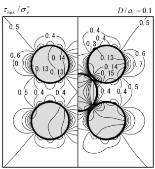
for the case of a single rigid inclusion (top figure) and three rigid inclusions (bottom figure) underσ∞y, when D/a1= 0.1 .
Fig. 10 Distribution ofτmaxfor the case of 4 and 5 soft inclusions underσ∞y.
Fig. 11 Distribution ofτmaxfor the case of 4 and 5 hard inclusions underσ∞y.
Fig. 10 shows the distribution ofτmaxfor the case of four soft inclusions (left figure) and
five soft inclusions (right figure) underσ∞y. In the case of five inclusions, the radii are all the same and the interference D/a1with each other is 0.1. The geometry in the case of the four
inclusions is the same as in the case of five inclusions. Fig. 11 shows the case of four hard inclusions (left figure) and five hard inclusions (right figure) when D/a1= 10.
Fig. 12 Distribution ofτmaxfor the case of 7 inclusions underσ∞y.
Fig. 13 Distribution ofτmaxfor the case of a RC with an air hole underσ∞y.
Fig. 12 shows the distribution ofτmaxfor the case of seven soft inclusions e= 0.1 (left
figure) and seven hard inclusions e= 10 (right figure) under σ∞y.
Finally, we show a realistic example so that we can consider the reinforced concrete problem underσ∞y in Fig. 13. In this problem, we replace the matrix with concrete and the inclusion with an iron reinforcing bar. The bottom figure shows that a dead air space having a radius a1/2 comes in contact with the two bars. When the distance of two bars is close, the air
space occurs easily. We may find high maximum shear stressτmaxaround the concrete near
4. Concluding Remarks
In the present paper, we examined the in-plane problem of a two-dimensional isotropic matrix containing many circular elastic inclusions subjected to arbitrary loading and produced general solutions to find the stresses and displacements. The purpose of this characteristic study was to apply Moriguchi’s reflection principle. Using these solutions, several numerical examples were presented graphically.
These problems have previously been solved using different numerical analysis methods such as the finite element method (FEM) and the boundary element method (BEM). However, our studies were developed in order to observe the interacting disturbances for many circular inclusions with high precision.
References
( 1 ) Moriguchi, S., Two Dimensional Elastic Theory (in Japanese), (1956), pp. 1-77, Iwatani Ltd.
( 2 ) J.Dunders, Elastic interaction of dislocations with inhomogeneities, in Mathematical Theory of Dislocations, edited by T.MURA, A.S.M.E.,(1969),pp. 70-115
( 3 ) G.P.Sendeckyj, ELASTIC INCLUSION PROBLEMS IN PLANE ELASTOSTATICS, Int.J.Solids Structure, Vol.6,(1970),pp. 1535-1543.
( 4 ) E.Honein, T. Honein, and G. Herrmann,ON TWO CIRCULAR INCLUSIONS IN HAR-MONIC PROBLEMS, QUARTERLY OF APPLIED MATHEMATICS, Vol.L, No.3 (1992), pp. 479-499.
( 5 ) Hirashima, K., and Sugisaka, N., Analytical Solution for Out-of-Plane Problems with Two Circular Elastic Inclusions, Transactions of the Japan Society of Mechanical Engi-neers, Series A, Vol. 60, No. 575 (1994), pp. 71-77.
( 6 ) Kimura, K., Hirashima, K., and Hirose, Y., Analytical Solutions for In-Plane and Out-of-Plane Problems with Elliptic Hole or Elliptic Rigid Inclusion and Their Applications Transactions of the Japan Society of Mechanical Engineers, Series A, Vol. 58, No. 555 (1992), pp. 94-100.
( 7 ) Hirashima, K., Miyagawa, M., and Nakane, S., Analysis of Antiplane Problems with Singular Disturbances for Isotropic Elastic Medium Having Many Circular Elastic In-clusions, Transactions of the Japan Society of Mechanical Engineers, Series A, Vol. 64, No. 623 (1998), pp. 143-150.
( 8 ) Miyagawa, M., Suzuki,T., and Shimura, J. , Analysis of In-Plane Problems with Singular Disturbances for Isotropic Elastic Medium Which Has Two Circular Holes or Rigid Inclusions, Transactions of the Japan Society of Mechanical Engineers, Series A, Vol. 75, No. 750 (2009), pp. 150-157.
( 9 ) Miyagawa, M., Tamiya, T., Shimura, J., and Suzuki, T., Analysis of In-Plane Problems for Isotropic Elastic Medium Which Has Two Circular Elastic Inclusions, Transactions of the Japan Society of Mechanical Engineers, Series A, Vol. 76, No. 762 (2010), pp. 136-144.
(10) Miyagawa, M., Shimura, J., Suzuki, T., and Tamiya, T., Analysis of In-Plane Prob-lems for Isotropic Elastic Medium Which Has Many Circular Holes or Rigid Inclusions, Transactions of the Japan Society of Mechanical Engineers, Series A, Vol. 77, No. 774 (2011), pp. 251-260.

![Fig. 5 Graph of the relative errors [RE] in the calculation of the n-count.](https://thumb-ap.123doks.com/thumbv2/123deta/6829197.1168201/13.892.390.708.683.1012/fig-graph-relative-errors-calculation-n-count.webp)