Article
Does Non-Fossil Energy Usage Lower CO
2
Emissions? Empirical Evidence from China
Deshan Li1,2,3and Degang Yang1,*
1 Xinjiang Institute of Ecology and Geography, Chinese Academy of Sciences, Urumqi 830011, China;
2 University of Chinese Academy of Sciences, Beijing 100049, China
3 Institute for the Economy of Xinjiang Production and Construction Corps, Urumqi 830002, China
* Correspondence: [email protected]; Tel.: +86-991-788-5346
Academic Editor: Andrew Kusiak
Received: 25 July 2016; Accepted: 26 August 2016; Published: 30 August 2016
Abstract:This paper uses an autoregressive distributed lag model (ARDL) to examine the dynamic impact of non-fossil energy consumption on carbon dioxide (CO2) emissions in China for a given
level of economic growth, trade openness, and energy usage between 1965 and 2014. The results suggest that the variables are in a long-run equilibrium. ARDL estimation indicates that consumption of non-fossil energy plays a crucial role in curbing CO2emissions in the long run but not in the short
term. The results also suggest that, in both the long and short term, energy consumption and trade openness have a negative impact on the reduction of CO2emissions, while gross domestic product
(GDP) per capita increases CO2emissions only in the short term. Finally, the Granger causality test
indicates a bidirectional causality between CO2emissions and energy consumption. In addition,
this study suggests that non-fossil energy is an effective solution to mitigate CO2emissions, providing
useful information for policy-makers wishing to reduce atmospheric CO2.
Keywords:non-fossil energy consumption; CO2emissions; ARDL model
1. Introduction
Climate change and global warming are among the most urgent environmental problems confronting modern societies, posing a growing threat to human survival and development. Greenhouse gas emissions, mainly containing carbon dioxide (CO2), represent the principal cause
of climate change. CO2primarily results from fossil fuels combustion for energy production and
transportation, producing about the 85% of global CO2 emissions. Thus, it is important to find
alternative energy sources to mitigate CO2emissions.
China has overtaken the USA as the biggest consumer of energy and largest contributor of CO2
emissions, with 20% of global energy consumption and 29% of total CO2emissions. The country relies
on fossil fuels, and in particular coal whose burning releases large amounts of CO2into the atmosphere,
as the main energy source. There are two main solutions to increasing energy consumption, greenhouse gas (GHGs) emission, and environmental pollution. One is to establish markets where emissions allowances can be traded and priced [1–4]. The other is to improve the proportion of renewable energy and nuclear resources in the energy structure.
To mitigate CO2 emissions while sustaining economic and social development, China has
undertaken initiatives to develop renewable and nuclear energy resources to replace traditional fossil fuels. The government has created energy policies to promote the use of clean energy. As a result, non-fossil energy consumption increased from 3.8% to 10.9% from 1965 to 2014. In addition, China plans to raise the share of non-fossil energy in the energy mix to around 20% by 2030.
Although the government has made great efforts to develop clean energy sources and obtained remarkable results, the effects of non-fossil energy on GHG emissions requires further empirical tests. There is a debate on whether non-fossil energy reduces carbon emissions, as their use may lead to extra emissions [5]. For example, greenhouse gas emissions for the life cycle of solar panels account for approximately 32–79 g CO2eq/kWh, while for solar collectors it is 11–68 g CO2eq/kWh [6]. Therefore,
this paper aims to assess whether an increase in the share of non-fossil energy would have a statistically significant effect on the reduction of CO2emissions.
Previous researchers investigated the contribution of non-fossil energy consumption to CO2
emissions. Most of these studies used different econometric methodologies to measure the effects of renewable and nuclear energy for emissions reduction. However, the results are contradictory and inconclusive.
Silva et al. [7] examined the causal relationship between renewable energy sources and CO2
emissions between 1960 and 2004 in the USA, Spain, Portugal, and Denmark, concluding that the increase in the proportion of renewable energy in the energy mix reduced CO2emissions in nearly all
countries except the USA. Al-Mulali et al. [8] found that renewable energy consumption cuts down on CO2emissions in Western, Central and Eastern Europe, East Asia and the Pacific, the Americas
and South Asia. Irandoust [9] provided evidence supporting that renewable energy mitigates CO2
emissions in four Nordic countries. Dogan and Seker [10] confirmed that expanding the use of renewable energy decreases CO2emissions in the top renewable energy countries. Bento et al. [11] and
Tiwari [12] arrived at the same conclusions for Italy and India; Bilgili et al. [13], Bölük and Mert [14], Saidi et al. [15], Sebri et al. [16], Özbu˘gday et al. [17], and Dogan et al. [18] provided similar results for 17 panel Organisation for Economic Co-operation and Development (OECD) countries, 16 European Union countries, nine developed countries, BRICS countries, thirty-six countries and the European Union, respectively.
However, Apergis et al. [19] noted that use of renewable energy does not affect carbon emission reduction in the short-run. Menyah and Rufael [20] explored the causal relationship between renewable energy consumption and CO2emissions in the US between 1960 and 2007, discovering that renewable
energy does not significantly contribute to the reduction of CO2emissions. Chiu and Chang [21] found
that the renewable energy will begin to mitigate CO2emissions when it represents at least 8.3889% of
the total energy supply.
As for nuclear energy, Al-mulali [22] found that it plays a major role in decreasing CO2emissions
in both the short and the long term, since it positively affects GDP growth without enhancing CO2emission. Baek [23] showed that nuclear energy and CO2emissions have a negative long-run
relationship in USA, France, Japan, Korea, Canada, and Spain. Nuclear energy has a favorable impact on mitigating CO2emissions in Korea, USA and in in 12 major nuclear generating countries [20,24–26].
On the contrary, Iwata et al. [27] concluded that nuclear energy plays a minimal role in curbing CO2emissions in most OECD countries. According to Jaforullah et al. [12], CO2emission are unrelated
to nuclear energy utilization in the USA when energy prices are not considered as a possible driving force of energy demand.
While numerous studies investigated the link between renewable energy, nuclear energy use, and CO2emissions, little empirical work examined the association between total non-fossil energy
consumption and CO2emissions employing modern econometric methods. In addition, the empirical
research largely focused on the short term impact of renewable and nuclear energy on CO2emissions.
Furthermore, to the best of our knowledge, few scholars investigated the effect of nuclear and renewable energy utilization on CO2emissions specifically in China.
To fill these gaps, this paper aims to study the dynamic effects of non-fossil energy utilization on CO2emissions within the cointegration framework. In particular, it investigates the short and long
term impacts of non-fossil energy, economic growth, energy consumption, and trade openness on CO2
2. Materials and Methods
2.1. Model Equation
To investigate the changes in CO2 emissions employing time-series data, Equation (1) took
into consideration variables that substantially affect CO2 emissions, as reported in previous
studies [15,18,20,25].
ln(co2)t=β0+β1lnn ft+β2lnyt+β3lnent+β4lntt+ut (1)
where (co2)trepresents CO2emissions at time t;nftis a measure of non-fossil energy consumption;
yt represents economic growth; ent represents energy consumption; tt is trade openness; and ut
represents the error term. If increasing non-fossil energy use results in a reduction on CO2emissions,
the coefficient of this variable would become negative. According to the literature, economic growth occupies a central role in affecting environmental quality; as economic development increases CO2
emissions, the sign ofβ2 could be expected to be positive. In addition, a higher level of energy
utilization should lead to an increase in CO2emissions, so the sign ofβ3could become positive. Finally,
as increasing trade openness will raise CO2emissions in developing countries, the coefficient of this
variable would become positive.
2.2. Cointegration Analysis
In order to examine the long term equilibrium relationship among non-fossil energy use, economic development, energy usage, trade openness, and CO2emissions, this study adopts an ARDL approach
developed by Pesaran and Shin [28]. This approach has some advantages compared to those of multivariate cointegration, as confirmed by Narayan [29]. The unrestricted error correction regressions representation of Equation (1) is expressed below:
△ln(co2)t=β0+
n ∑ k=1
β1k△ln(co2)t−k+ n ∑ k=0
β2k△lnn ft−k+ n ∑ k=0
β3k△lnyt−k+ n ∑ k=0
β4k△lnent−k
+∑n
k=0β5k△lntt−k+ϕ0ln(co2)t−1+ϕ1lnn ft−1+ϕ2lnyt−1+ϕ3lnent−1+ϕ4lntt−1+νt
(2)
where ∆ is the first difference of the variable, β is the intercept term, and parameter n represents the lag lengths. The proper lag length is selected based on the Akaike information criterion (AIC) or final prediction error (FPE). The F-test proposed by Pesaran et al., which is highly sensitive to lag order selection, is suitable to determine the joint significance of the coefficients of the lagged level of the variables [30]. The null hypothesis of no long run relationship (H0:ϕ0=ϕ1 =ϕ2=ϕ3=ϕ4 =0) should be tested against the alternative hypothesis
(H1: ϕ0 6= ϕ1 6= ϕ2 6= ϕ3 6= ϕ4 6= 0). F-statistics are compared to the critical bounds reported
in Pesaran et al. [30]. If the test result exceeds the upper critical value, it means that the null hypothesis is rejected. If the calculated F-statistic is between the upper and lower critical bounds, it implies the test is inconclusive. However, if the test statistic is below the lower bounds value, it means there is no cointegration.
After examining the long term relation among variables, the next step is to continue to estimate the long term coefficient of the ARDL model by using Equation (3).
ln(co2)t=β0+ n ∑ k=1
β1kln(co2)t−k+ n1
∑ k=0
β2klnn ft−k+ n2
∑ k=0
β3klnyt−k+ n3
∑ k=0
β4klnent−k
+n∑4 k=0
β5klntt−k+µ1t
When this procedure is completed, Equation (4) estimates the error-correction model examining the short term behaviors of the variables together with the short term adjustment speed towards long term speed.
△ln(co2)t=β0+ ∑n
k=1β1k△ln(co2)t−k+
n ∑
k=0β2k△lnn ft−k+
n ∑
k=0β3k△lnyt−k+
n ∑
k=0β4k△lnent−k +∑n
k=0
β5k△lntt−k+ηectt−1+µ1t
(4)
Finally, to avoid instability caused by the parameter set resulting in an unreliable model, a stability test is necessary for the resulting estimated parameters. The cumulative sum of recursive residuals (CUSUM) and cumulative sum of squares of recursive residuals (CUSUMSQ) tests [31] are used to examine the stability of the coefficients. Both tests were carried out at the 5% significance level. If the plots of the CUSUM and CUSUMSQ statistics remain within the 5% significance interval, the null hypothesis cannot be rejected, indicating that all coefficients in the given regression are stable.
2.3. Granger Causality Test
The existence of cointegration indicates a causal relation between variables, but the direction of causality is unclear. Therefore, the Granger causality test [32] is used to investigate short and long term causal dynamics among variables. If the variables are non-stationary and there is a cointegration relationship between them, Equation (5) develops a vector error correction model to test for Granger causality between variables:
(1−L)
co2t n ft yt ent tt = c1 c2 c3 c4 c5 + q ∑ i=1(1−L)
a11ia12ia13ia14ia15i a21ia22ia23ia24ia25i a31ia32ia33ia34ia35i a41ia42ia43ia44ia45i a51ia52ia53ia54ia55i
co2t−1
n ft−1
yt−1
ent−1
tt−1 + λ1 λ2 λ3 λ4 λ5
[ECTt−1] +
δ1t δ2t δ3t δ4t δ5t
(5) 2.4. Data
Annual observations were collected between 1965–2014. CO2emissions were measured using
total CO2emissions (measured in millions of metric tons). Non-fossil energy, including nuclear and
renewable energy (hydroelectric, solar, wind, biomass, and geothermal), is measured in millions of tons of oil equivalent. These data are collected from the BP Statistical Review of World Energy. Real GDP per capita is measured in constant 2005 USD. Energy consumption is measured using total primary energy consumption per capita (measured as kg of oil equivalent per capita). The data for these two variables were collected from the World Bank. Trade openness is measured as [(exports + imports)/GDP]. These data were obtained from the China statistical yearbooks. TableA1summarizes descriptive statistics of each variable used in estimating Equation (1). The descriptive statistics of the growth rates of the variables are shown in TableA2.
3. Results
3.1. Unit Root Tests
but all series were stationary after taking the first difference at 1% level (Table1). Based on this result, ARDL appears to be a suitable method for a cointegration test.
Table 1.Results of unit root test.
Variable Level First Difference
SIC Lag DFGLS Stat SIC Lag DFGLS Stat Decision
ln(co2)t 1 0.469 0 −3.827 *** I(1)
lnnft 0 3.817 0 −6.085 *** I(1)
lnyt 1 1.163 1 −4.590 *** I(1)
lnent 1 −0.017 0 −3.921 *** I(1)
lntt 0 −0.391 0 −5.385 *** I(1)
Note: Stars indicate statistical significance. *** 1% level.
3.2. ARDL Cointegration Method
Since the choice of lag length can affect theF-test, it is necessary to select the proper lag order of the variables prior to employing ARDL bounds testing. Application of the following system-wide methods determines the optimal lag order: Akaike information criterion (AIC), Final Prediction Error (FPE) criterion, Hannan-Quinn (HQ) criterion and Schwarz information criterion (SIC), and likelihood ratio (LR). The test results indicated that the optimal lag length is three (Table2).
Table 2.Lag order selection criteria.
Lag LogL LR FPE AIC SC HQ
0 54.783 NA 1.29×10⁻⁶ −2.207 −2.0489 −2.1484
1 334.788 499.139 1.34×10⁻¹¹ −13.686 −12.8913 −13.388
2 367.490 52.608 6.60×10⁻¹² −14.412 −12.981 * −13.876 *
3 388.865 30.668 * 5.45×10−12* 14.646 * −12.579 −13.871
4 399.251 13.096 7.57×10⁻¹² −14.402 −11.699 −13.389
Note: * indicates the lag order selected by the criterion. LR, Likelihood Ratio; FPE, Final Prediction Error; AIC, Akaike Information Criterion; HQ, Hannan-Quinn criterion; SIC, Schwarz Information Criterion.
After determining the optimal lag order, this study applied the F-test to probe the cointegrating relationship among variables. The results indicated that theF-statistics exceeded the upper critical bound at the 1%, 5%, and 10% levels with CO2as a dependent variable (Table3). According to the
suggestion by Pesaran et al. [30], the null hypothesis of no long run relationship is rejected. ARDL bounds testing confirmed that these variables are cointegrated for a long term relation among non-fossil energy usage, economic development, energy consumption, trade openness, and CO2emissions.
Having identified the existence of a long run relationship between the variables, Equation (3) estimates the long-run coefficient (Table 4). The coefficient of lnnft is negative and significant,
suggesting that non-fossil energy consumption decreases CO2emissions in the long term. For example,
a 1% increase in non-fossil energy utilization leads to a 0.051% decrease in CO2emissions.
The coefficient of lnyt is negative but statistically insignificant, implying that CO2 emissions
initially declined with an increase in per capita GDP. This conclusion is consistent with what was previously reported for Malaysia [34]. The coefficient of lnentis statistically significant and positive,
implying that energy consumption per capita increases CO2emissions in the long term. It should be
noted that a 1% increase in energy usage increases CO2emissions by 0.560%. This is in agreement with
Table 3.Results of the bounds tests of Equation (2).
Panel I: Bounds Testing of Cointegration Panel II: Diagnostic Tests
Estimated equation ln(co2)t= f(lnnft, lnyt, lnent, lntt) R2 0.858
Optimal lag
structure (3, 1, 1, 0) Adjusted-R2 0.814
F-statistics
(Wald-statistics) 4.480
F-statistics
(prob-value) 19.325 (0.000) ***
Significant level Critical values (T = 47) Durbin–Watson 0.963
Lower bounds, I(0) Lower bounds, I(1) J–B normality test 0.341 (0.926)
1% 3.74 5.06 Breusch-Godfrey
LM test 1.593 (0.375)
5% 2.86 4.01 ARCH LM test 1.476 (0.348)
10% 2.45 3.52 Ramsey RESET 0.387 (0.982)
Note: Stars indicate statistical significance. *** 1% level.
Table 4.Long-run coefficient estimates.
Variable Coefficient Standard Error t-Statistic Prob.
lnnft −0.051 ** 0.123 −1.233 0.002
lnyt −0.145 0.126 −1.186 0.243
lnent 0.560 *** 0.077 7.283 0.000
lntt 1.203 *** 0.194 6.22 0.000
Constant 3.447 *** 0.695 4.961 0.000
Note: Stars indicate statistical significance. *** 1% level; ** 5% level.
Trade openness positively correlates with CO2emissions and it is statistically significant at the 1%
level. A 1% increase in trade openness causes a 1.203% increase in CO2emissions. This is in agreement
with previous work form Tao and Song [41], but it contradicts Shahbaz et al. [42] for the case of Tunisia and Shahbaz et al. [43] for Indonesia, which showed that trade openness allows developing economies access to advanced technologies, resulting in a reduction of CO2emissions.
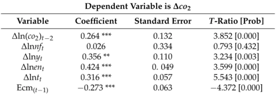
The error correction model is estimated on the base of SIC (Table5). The elasticity of CO2
emissions for non-fossil energy usage was positive in the short run and statistically insignificant at conventional levels. This finding provides little evidence on the beneficial role of non-fossil energy usage on CO2emissions in the short term. However, non-fossil energy usage has a positive impact on
the environment in the long term, likely because non-fossil energy usage reaches a level that affects CO2emissions.
Table 5.Error correction representation of the autoregressive distributed lag (ARDL) model.
Dependent Variable is∆co2
Variable Coefficient Standard Error T-Ratio [Prob]
∆ln(co2)t−2 0.264 *** 0.132 3.852 [0.000]
∆lnnft 0.026 0.334 0.793 [0.432]
∆lnyt 0.356 ** 0.110 3.234 [0.003]
∆lnent 0.424 *** 0. 049 3.599 [0.000]
∆lntt 0.316 *** 0.057 5.543 [0.000]
Ecm(t−1) −0.273 *** 0.063 −4.372 [0.000]
Economic growth has a positive and statistically significant effect on CO2emissions at the 1%
level in the short run, implying that a GDP per capita increase of 1% raises CO2emissions by 0.356%.
The short-run elasticity of energy usage for CO2emissions is 0.424, indicating that a 1% increase in per
capita energy usage is related with a 0.424% increase in CO2emissions. Thus, energy usage seems to
be an important factor in environmental degradation after economic growth in the short run.
The result suggests that a positive relationship between trade openness and CO2emissions exists
in the short term at the 1% level. For example, a 1% increase in trade openness causes a 0.316% increase in CO2emissions in the short run. This is similar to the findings in Shahbaz et al. [44] for the case of
Bangladesh. The error-correction term reveals the CO2adjustment rate back to its long-run equilibrium
level after a shock. The error-correction term is statistically significant and negative. The estimated coefficient of Ecm(t−1)is−0.273, which suggests that the deviation from the long-run balanced level of
CO2emissions in one year is adjusted by 27.3% over the next year.
3.3. The VECM Granger Causality Results
Table 6 displays the results of the Granger causality analysis. In the short run, there is a unidirectional relationship from non-fossil energy use to energy consumption and CO2emissions,
suggesting a Granger-causality relationship with non-fossil energy use causing energy consumption and CO2emissions in the short term. These findings imply that the construction and maintenance of
non-fossil energy generation facilities may result in energy consumption and additional emissions. A unidirectional relationship from GDP per capita to CO2emissions exists, too, indicating that GDP
per capita causes CO2emissions in the short run. This result is in agreement with Shafiei and Salim [45]
for the case of OECD countries but contrasts with Salim and Rafiq [46] for India, which indicates unidirectional causality from CO2emissions to income. It also differs from Xue et al. [47] for nine
European countries and Peng et al. [48] for China. In addition, there is a unidirectional relationship from GDP per capita to energy consumption and from CO2emissions to trade openness. This implies
that emission mitigation policies would influence trade openness in the short term.
Table 6.Granger causality test.
Short-RunF-Statistics (Probability) Long Run Dependent
Variable ∆ln(co2)t ∆lnnft ∆lnyt ∆lnent ∆lntt
Ectt−1 (t-Statistics)
∆ln(co2)t — 7.378 **(0.025) 13.471 ***(0.001) 11.213 ***(0.004) 3.989 (0.136) −0.61(3.28) **
∆lnnft 0.520 (0.770) — 2.695 (0.259) 0.845 (0.655) 1.054 (0.590)
∆lnyt 0.871 (0.647) 2.334 (0.311) — 1.435 (0.487) 0.020 (0.989) —
∆lnent 16.870 *** (0.000)
13.610 *** (0.001)
8.370 **
(0.015) — 2.191 (0.334) —
∆lntt (0.052)5.924 * 1.709 (0.425) 1.104 (0.575) 4.055 (0.132) —
Note: Stars indicate statistical significance. *** 1% level; ** 5% level; * 10% level.
Carbon dioxide emissions have a significant influence on energy consumption and vice versa, suggesting a bidirectional relationship between them. These data are consistent with those of Halicioglu [49] for Turkey and Tang and Tan [50] for Vietnam, but they contradict Soytas and Sari [51], which suggests that there is only a one-way causal relationship from CO2emissions to energy use.
3.4. Instability Tests Results
To avoid the instability caused by the parameter set leading to an unreliable model, this study employs CUSUM and CUSUMSQ to test the stability for the parameters used for the model. Every coefficient in the constructed error-correction model is stable and credible, with the plots of both tests well within the critical bounds at the 5% significance level (Figures1and2). Thus, the chosen model can be applied to policy decision-making purposes, so that the effect of policy changes considering economic growth, energy consumption, trade openness, and non-fossil energy consumption would not result in major distortions in the level of CO2, as the parameters in this model follow a stable pattern
over the period under examination.
-20 -10 0 10 20
1968 1980 1992 2004 2014
The straight lines represent critical bounds at 5% significance level
Plot of Cumulative Sum of Recursive Residuals
Figure 1. Figure 1.Recursive residuals and cumulative test results.Recursive residuals and cumulative test results.
-0.4 -0.2 0.0 0.2 0.4 0.6 0.8 1.0 1.2 1.4
1968 1980 1992 2004 2014
The straight lines represent critical bounds at 5% significance level
Plot of Cumulative Sum of Squares of Recursive Residuals
Figure 2. Figure 2.Recursive cumulative sum of squared residuals and test results.Recursive cumulative sum of squared residuals and test results.
4. Conclusions and Policy Implications
China is faced with the environmental challenge to reduce its dependency on fossil fuels in order to substantially diminish its CO2emissions. As alternatives to traditional energy, non-fossil
energy usage is an effective means of mitigating climate change. This study investigates the long term relationship among CO2emissions, economic development, non-fossil energy usage, energy
consumption, and trade openness by using an ARDL model. The short term relationship dynamics were examined using ECM.
The results confirmed that there is both a long- and short-run relationship between CO2emissions,
non-fossil energy consumption, energy consumption, economic development, and trade openness. Non-fossil energy usage reduces CO2emissions with a significant effect in the long run. This study
finds that non-fossil energy consumption has a major part to play in curbing CO2emissions in the
emissions both in the long and short term. However, GDP per capita does not have any remarkable impact on CO2emissions in the long term but increases them in the short term. Therefore, the results
prove that CO2emissions are mainly determined by economic development, trade openness, and
energy use in the short term. The Granger causality test shows one-way causal relationship from non-fossil energy usage to CO2emissions. Other one-way causal relationships from GDP per capita
to energy use and from CO2emissions to trade openness were also confirmed. Moreover, there is
bidirectional causality between CO2emissions and energy usage.
These results have important implications for policy making. Specifically, the results indicate that the country’s energy usage and corresponding CO2emissions will continue to grow over the long
term in the coming decades. To reduce pollution as well as achieve economic stability and sustainable growth, it is necessary to continue increasing the share of renewable energy and reduce dependency on fossil fuels. For example, the government should formulate and implement effective policies to promote technology innovation in renewable and nuclear energy. It should also devote more attention to the subsidy system for clean energy prices and improve the pricing mechanisms for solar and wind power, as well as power generated from other non-fossil sources. It would also be necessary to introduce tax policies that encourage investments in non-fossil power generation, transmission and storage. Furthermore, the government should pay more attention to the effects of environmental deterioration resulting from increased trading activities. It is necessary to encourage enterprises to introduce advanced foreign technologies and managerial experience in the fields of environmental protection and clean manufacturing. The administration should also enhance environmental supervision of foreign-funded enterprises.
Author Contributions:All the authors have been involved in the work of the paper. Deshan Li conceived and designed the experiments; Deshan Li composed the manuscript, while Degang Yang revised it. Both authors read the final version and agreed with its content.
Conflicts of Interest:The authors claim that there is no conflict of interest.
Appendix A
Table A1.Descriptive statistics for the variables.
Variable Mean Std. Dev. Min Max
co2 3343.539 2788.524 476.772 9761.078
en 882.814 534.209 167.418 2230.150
nf 59.868 76.407 4.386 322.534
t 0.284 0.185 0.050 0.653
y 950.773 1044.298 109.384 3862.917
Table A2.Descriptive statistics for the growth rates of the variables.
Variable Mean Std. Dev. Min Max
co2 0.065 0.064 −0.102 0.286
en 0.057 0.115 −0.123 0.695
nf 0.092 0.087 −0.138 0.297
t 0.046 0.136 −0.222 0.389
y 0.075 0.048 −0.081 0.162
References
1. Daskalakis, G.; Psychoyios, D.; Markellos, R.N. Modelling CO2Emission Allowance Prices and Derivatives:
Evidence from the European Trading Scheme.J. Bank. Financ.2009,33, 1230–1241. [CrossRef]
3. Oestreich, A.M.; Tsiakas, I. Carbon emissions and stock returns: Evidence from the EU Emissions Trading Scheme.J. Bank Financ.2015,58, 294–308. [CrossRef]
4. Salant, S.W. What ails the European Union’s emissions trading system? J. Environ. Econ. Manag. 2016. [CrossRef]
5. Jaforullah, M.; King, A. Does the use of renewable energy sources mitigate CO2, emissions? A reassessment
of the US evidence.Energy Econ.2015,49, 711–717. [CrossRef]
6. Sokka, L.; Sinkko, T.; Holma, A.; Manninen, K.; Pasanen, K.; Rantala, M.; Leskinen, P. Environmental impacts of the national renewable energy targets—A case study from Finland.Renew. Sustain. Energy Rev.2016,59, 1599–1610. [CrossRef]
7. Silva, S.; Soares, I.; Pinho, C. The Impact of Renewable Energy Sources on Economic Growth and CO2 Emissions—A SVAR Approach.Eur. Res. Stud.2012,15, 133–144.
8. Al-Mulali, U.; Solarin, S.A.; Ozturk, I. Investigating the environmental Kuznets curve hypothesis in seven regions: The role of renewable energy.Ecol. Indic.2016,67, 267–282. [CrossRef]
9. Irandoust, M. The renewable energy-growth nexus with carbon emissions and technological innovation: Evidence from the Nordic countries.Ecol. Indic.2016,69, 118–125. [CrossRef]
10. Dogan, E.; Seker, F. The influence of real output, renewable and non-renewable energy, trade and financial development on carbon emissions in the top renewable energy countries.Renew. Sustain. Energy Rev.2016, 60, 1074–1085. [CrossRef]
11. Bento, J.P.C.; Moutinho, V.M.F. CO2 emissions, non-renewable and renewable electricity production,
economic growth, and international trade in Italy.Renew. Sustain. Energy Rev.2016,55, 142–155. [CrossRef] 12. Tiwari, A.K. A Structural VAR Analysis of Renewable Energy Consumption, Real GDP and CO2Emissions:
Evidence from India.Econ. Bull.2011,31, 1793–1806.
13. Bilgili, F.; Koçak, E.; Bulut, Ü. The dynamic impact of renewable energy consumption on CO2emissions: A
revisited Environmental Kuznets Curve approach.Renew. Sustain. Energy Rev.2016,54, 838–845. [CrossRef] 14. Bölük, G.; Mert, M. Fossil & renewable energy consumption, GHGs (greenhouse gases) and economic
growth: Evidence from a panel of EU (European Union) countries.Energy2014,74, 439–446.
15. Saidi, K.; Mbarek, M.B. Nuclear energy, renewable energy, CO2emissions, and economic growth for nine
developed countries: Evidence from panel Granger causality tests. Prog. Nucl. Energy2016,88, 364–374. [CrossRef]
16. Sebri, M.; Ben-Salha, O. On the causal dynamics between economic growth, renewable energy consumption, CO2, emissions and trade openness: Fresh evidence from BRICS countries.Renew. Sustain. Energy Rev.2014,
39, 14–23. [CrossRef]
17. Özbu˘gday, F.C.; Erbas, B.C. How effective are energy efficiency and renewable energy in curbing CO2,
emissions in the long run? A heterogeneous panel data analysis.Energy2015,82, 734–745. [CrossRef] 18. Dogan, E.; Seker, F. Determinants of CO2, emissions in the European Union: The role of renewable and
non-renewable energy.Renew. Energy2016,94, 429–439. [CrossRef]
19. Apergis, N.; Payne, J.E.; Menyah, K.; Wolde-Rufael, Y. On the causal dynamics between emissions, nuclear energy, renewable energy, and economic growth.Ecol. Econ.2010,69, 2255–2260. [CrossRef]
20. Menyah, K.; Wolde-Rufael, Y. CO2, emissions, nuclear energy, renewable energy and economic growth in
the US.Energy Policy2010,38, 2911–2915. [CrossRef]
21. Chiu, C.L.; Chang, T.H. What proportion of renewable energy supplies is needed to initially mitigate CO2,
emissions in OECD member countries?Renew. Sustain. Energy Rev.2009,13, 1669–1674. [CrossRef] 22. Al-Mulali, U. Investigating the impact of nuclear energy consumption on GDP growth and CO2, emission:
A panel data analysis.Prog. Nucl. Energy2014,73, 172–178. [CrossRef]
23. Baek, J.; Pride, D. On the Income-Nuclear energy-CO2Emissions Nexus Revisited.Energy Econ.2014,43,
6–10. [CrossRef]
24. Baek, J.; Kim, H.S. Is economic growth good or bad for the environment? Empirical evidence from Korea. Energy Econ.2013,36, 744–749. [CrossRef]
25. Baek, J. Do nuclear and renewable energy improve the environment? Empirical evidence from the United States.Ecol. Indic.2016,66, 352–356. [CrossRef]
27. Iwata, H.; Okada, K.; Samreth, S. Empirical study on the determinants of CO2emissions: Evidence from
OECD countries.Appl. Econ.2010,44, 3513–3519. [CrossRef]
28. Pesaran, M.H.; Shin, Y.An Autoregressive Distributed Lag Modeling Approach to Co-Integration Analysis; Cambridge University Press: Cambridge, UK, 1995; pp. 371–413.
29. Narayan, P.K. The saving and investment nexus for China: Evidence from cointegration tests.Appl. Econ.
2005,37, 1979–1990. [CrossRef]
30. Pesaran, M.H.; Smith, R.J.; Shin, Y. Bound Testing Approaches to the Analysis of Level Relationships. J. Appl. Econ.2001,16, 289–326. [CrossRef]
31. Pesaran, M.H.; Pesaran, B.Working with Microfit 4.0: Interactive Econometric Analysis; Oxford University Press: Oxford, UK, 1997.
32. Granger, C.W.J. Investigating Causal Relations by Econometric Models and Cross-Spectral Methods. Econometrica1969,37, 424–438. [CrossRef]
33. Elliott, G.; Rothenberg, T.J.; Stock, J.H. Efficient Tests for an Autoregressive Unit Root.Econometrica1996,64, 813–836. [CrossRef]
34. Begum, R.A.; Sohag, K.; Abdullah, S.M.S.; Jaafar, M. CO2, emissions, energy consumption, economic and
population growth in Malaysia.Renew. Sustain. Energy Rev.2015,41, 594–601. [CrossRef]
35. Friedl, B.; Getzner, M. Determinants of CO2emissions in a small open economy.Ecol. Econ.2003,45, 133–148.
36. Ang, J.B. CO2, emissions, energy consumption, and output in France. Energy Policy2007,35, 4772–4778. [CrossRef]
37. Ang, J.B. Determinants of foreign direct investment in Malaysia.J. Policy. Model.2008,30, 185–189. [CrossRef] 38. Shahbaz, M. Does financial instability increase environmental degradation? Fresh evidence from Pakistan.
Econ. Model.2013,33, 537–544. [CrossRef]
39. Liu, Q. Impacts of oil price fluctuation to China economy.Quant. Tech. Econ.2005,3, 17–28.
40. Jalil, A.; Feridun, M. The impact of growth, energy and financial development on the environment in China: A cointegration analysis.Energy Econ.2011,33, 284–291. [CrossRef]
41. Tao, H.Q.; Song, X.D. A Study on the Relationship of CO2 Emissions, Energy Consumption, Economic Growth, and Trade Openness in China—Analys is Based on ARDL Model.South China J. Econ.2010,10, 49–60. (In Chinese)
42. Shahbaz, M.; Lean, H.H. Does financial development increase energy consumption? The role of industrialization and urbanization in Tunisia.Energy Policy2012,40, 473–479. [CrossRef]
43. Shahbaz, M.; Hye, Q.M.A. Economic growth, energy consumption, financial development, international trade and CO2, emissions in Indonesia.Renew. Sustain. Energy Rev.2013,25, 109–121. [CrossRef]
44. Shahbaz, M.; Uddin, G.S.; Rehman, I.U.; Imran, K. Industrialization, electricity consumption and CO2,
emissions in Bangladesh.Renew. Sustain. Energy Rev.2014,31, 575–586. [CrossRef]
45. Shafiei, S.; Salim, R.A. Non-renewable and renewable energy consumption and CO2emissions in OECD
countries: A comparative analysis.Energy Policy2014,66, 547–556. [CrossRef]
46. Salim, R.A.; Rafiq, S. Why do some emerging economies proactively accelerate the adoption of renewable energy?Energy Econ.2012,34, 1051–1057. [CrossRef]
47. Xue, B.; Geng, Y.; Müller, K.; Lu, C.; Ren, W. Understanding the Causality between Carbon Dioxide Emission, Fossil Energy Consumption and Economic Growth in Developed Countries: An Empirical Study. Sustainability2014,6, 1037–1045. [CrossRef]
48. Peng, H.; Tan, X.; Li, Y.; Hu, L. Economic Growth, Foreign Direct Investment and CO2Emissions in China:
A Panel Granger Causality Analysis.Sustainability2016,8, 233. [CrossRef]
49. Halicioglu, F. An econometric study of CO2, emissions, energy consumption, income and foreign trade in
Turkey.Energy Policy2009,37, 1156–1164. [CrossRef]
50. Tang, C.F.; Tan, B.W. The impact of energy consumption, income and foreign direct investment on carbon dioxide emissions in Vietnam.Energy2015,79, 447–454. [CrossRef]
51. Soytas, U.; Sari, R. Energy consumption, economic growth, and carbon emissions: Challenges faced by an EU candidate member.Ecol. Econ.2009,68, 1667–1675. [CrossRef]