量子モデルと確率モデルの確率計算の違いによって生じる計算能力
の差について
天野 正己
(Masami Amano)
京都大学大学院情報学研究科
岩間 一雄
(Kazuo Iwama)
京都大学大学院情報学研究科
Abstract
The main
purpose
of this paper is to show that
we
can
ex-$\mathrm{i}\mathrm{t}\mathrm{y}\mathrm{c}\mathrm{a}1\mathrm{c}\mathrm{u}11\mathrm{a}\mathrm{t}\mathrm{i}\mathrm{o}\mathrm{n}\mathrm{b}\mathrm{e}\mathrm{t}\mathrm{w}\mathrm{e}\mathrm{e}\mathrm{n}\mathrm{q}\mathrm{u}\mathrm{a}\mathrm{n}\mathrm{t}\mathrm{u}\mathrm{m}\mathrm{a}\mathrm{n}\mathrm{d}\mathrm{p}\mathrm{r}\mathrm{o}l_{\mathrm{a}\mathrm{b}\mathrm{i}1\mathrm{i}\mathrm{s}\mathrm{t}\mathrm{i}\mathrm{c}\mathrm{c}\mathrm{o}\mathrm{m}\mathrm{p}\mathrm{u}-}^{\mathrm{i}\mathrm{n}\mathrm{t}\mathrm{h}\mathrm{e}\mathrm{p}\mathrm{r}\mathrm{o}\mathrm{b}\mathrm{a}\mathrm{b}\mathrm{i}1-}\mathrm{P}^{1\mathrm{o}\mathrm{i}\mathrm{t}\mathrm{t}\mathrm{h}\mathrm{e}\mathrm{d}\mathrm{i}\mathrm{f}\mathrm{f}\mathrm{e}\mathrm{r}\mathrm{e}\mathrm{n}\mathrm{c}\mathrm{e}(l_{1}\mathrm{n}\mathrm{o}\mathrm{r}\mathrm{m}\mathrm{a}\mathrm{n}\mathrm{d}l_{2}- \mathrm{n}\mathrm{o}\mathrm{r}\mathrm{m}}$
tations
to
claim the
difference
in
their
computational
pow-ers.
It is shown that there is
alanguage
$L$
which
contains
sentences
of length
up
to
$O(n^{\mathrm{c}+1})$
such that: (i) There
is
aone
way
quantum
finite
automaton
(qfa)
of
$O(n^{\mathrm{c}+4})$
states which recognizes L.
$(\dot{\iota}i)$However,
if
we
try to
sim-ulate this qfa by aprobabilistic finite
automaton
(pfa)
$\mathrm{I}\mathrm{t}\mathrm{s}\mathrm{h}\circ \mathrm{u}1\mathrm{d}\mathrm{b}\mathrm{e}\mathrm{n}\mathrm{o}\mathrm{t}\mathrm{e}\mathrm{d}\mathrm{t}\mathrm{h}\mathrm{a}\mathrm{t}\mathrm{w}\mathrm{e}\mathrm{d}\mathrm{o}\mathrm{n}\mathrm{o}\mathrm{t}\mathrm{p}\mathrm{r}\mathrm{o}\mathrm{v}\mathrm{e}\mathrm{r}\mathrm{e}\mathrm{a}\mathrm{f}_{1\mathrm{o}\mathrm{w}\mathrm{e}\mathrm{r}\mathrm{b}\mathrm{o}\mathrm{u}\mathrm{n}\mathrm{d}_{8}}^{n^{2\mathrm{c}+4})\mathrm{s}\mathrm{t}\mathrm{a}\mathrm{t}\mathrm{e}8}usingthesamedgo\dot{n}thm,\mathrm{t}\mathrm{h}\mathrm{e}\mathrm{n}\mathrm{i}\mathrm{t}\mathrm{n}\mathrm{e}\mathrm{e}\mathrm{d}_{8}\Omega$
.
for pfa’s
but show
that if pfa’s and qfa’s
use
exactly the
same
algorithm, then qfa’s need much less states.
1Introduction
It is well
known that BPP
can
be simulated by BQP
al-most directly,
i.e.,
quantum computation
with
abounded
error
is at least
as
powerful
as
its probabilistic counterpart
[BV97]. Furthermore, it
appears
that quantum
compu-tation
$\mathrm{h}\mathrm{a}\epsilon$ $8\mathrm{e}\mathrm{v}\mathrm{e}\mathrm{r}\mathrm{a}\mathrm{l}$merits
over
probabilistic computation,
which
include:
(t)
Quantum computation efficiently gives
us
useful
information about the period of
a
periodic
func-$\mathrm{a}\mathrm{r}\mathrm{e}4_{1\mathrm{o}\mathrm{w}\mathrm{e}\mathrm{d}’}^{\mathrm{s}\mathrm{h}\circ 94}\mathrm{t}\mathrm{i}\mathrm{o}\mathrm{n},$ $\mathrm{S}\mathrm{i}\mathrm{m}94].(\dot{|}i)\mathrm{N}\mathrm{e}\mathrm{g}\mathrm{a}\mathrm{t}\mathrm{i}\mathrm{v}\mathrm{e}\mathrm{v}\mathrm{a}\mathrm{l}\mathrm{u}\mathrm{e}8\mathrm{f}\mathrm{o}\mathrm{r}\mathrm{a}\mathrm{m}\mathrm{p}\mathrm{l}\mathrm{i}\mathrm{t}\mathrm{u}\mathrm{d}\mathrm{e}\mathrm{s}\mathrm{w}\mathrm{h}\mathrm{i}\mathrm{c}\mathrm{h}\mathrm{c}\mathrm{a}\mathrm{n}\mathrm{b}\mathrm{e}\mathrm{u}\mathrm{s}\mathrm{e}\mathrm{d},\mathrm{f}\mathrm{o}\mathrm{r}\mathrm{i}\mathrm{n}\mathrm{s}\mathrm{t}\mathrm{a}\mathrm{n}\mathrm{c}\mathrm{e},\mathrm{t}\mathrm{o}\mathrm{c}\mathrm{a}\mathrm{n}\mathrm{c}\mathrm{e}\mathrm{l}$
allows
us
to
do tricky operations by rotating the complex
number appropriately [AF98].
In this
paper,
we
focus
our
attention
on more
basic fea
ture
of quantum computation which has
been
relatively
less
focused
on
in
the
literature,
namely,
the difference in
the
way
of probability calculation. It is afundamental rule
of quantum computation that if astate
$q$
has
an
ampli-tude of
$\sigma$,
then
$q$
will
be observed not
with probability
$\sigma$but with probability
$\sigma^{2}$.
Suppose that there
are
ten pairs
of
state
$(p_{1}, q_{1})$
,
$\cdots$
,
$(p_{10}, q_{1}\mathrm{o})$
where,
for
each
$1\leq i\leq 10$
,
$\mathrm{e}\mathrm{i}\mathrm{t}\mathrm{h}\mathrm{e}\mathrm{r}\mathrm{i}\mathrm{s}\mathrm{O}\mathrm{N}$
if
$\mathrm{i}\mathrm{t}\mathrm{h}\mathrm{a}\S \mathrm{t}\mathrm{h}\mathrm{e}\mathrm{a}\mathrm{m}\mathrm{p}\mathrm{l}\mathrm{i}\mathrm{t}\mathrm{u}\mathrm{d}\mathrm{e}\mathrm{a}\mathrm{n}\mathrm{d}\mathit{4}_{\mathrm{F}\mathrm{F}\circ \mathrm{t}\mathrm{h}\mathrm{e}\mathrm{r}\mathrm{w}\mathrm{i}\mathrm{s}\mathrm{e}.).\mathrm{W}\mathrm{e}}^{\sqrt{10}(\mathrm{w}\mathrm{e}\mathrm{s}\mathrm{a}\mathrm{y}\mathrm{t}\mathrm{h}\mathrm{a}\mathrm{t}p_{\dot{1}}}\mathrm{a}\mathrm{n}\mathrm{d}q_{\dot{1}}\mathrm{h}\mathrm{a}8\mathrm{t}\mathrm{h}\mathrm{e}\mathrm{a}\mathrm{m}\mathrm{i}\mathrm{t}\mathrm{u}\mathrm{d}\mathrm{e}1$wish
to
know
how many
$p$
:’s
are
ON.
This
can
be done
by
“gathering” amplitudes by applying
a
Fourier
trans-fo
$\mathrm{r}$from
$p” \mathrm{s}$to
$r$
:
’s and observing
$\mathrm{r}\mathrm{i}\mathrm{o}$(see
later sections
$r_{10}\mathrm{a}\mathrm{f}\mathrm{f}\mathrm{i}\mathrm{e}\mathrm{r}d_{\mathrm{o}\mathrm{u}\mathrm{r}\mathrm{i}\mathrm{e}\mathrm{r}\mathrm{t}\mathrm{r}\mathrm{a}\mathrm{n}\mathrm{s}\mathrm{f}\mathrm{o}\mathrm{r}\mathrm{m}\mathrm{i}8\mathrm{o}\mathrm{n}\mathrm{e}\mathrm{a}\mathrm{n}\mathrm{d}\mathrm{i}\mathrm{t}\mathrm{i}\mathrm{s}\mathrm{o}\mathrm{b}\mathrm{s}\mathrm{e}\mathrm{r}\mathrm{v}\mathrm{e}\mathrm{d}\mathrm{w}\mathrm{i}\mathrm{t}\mathrm{h}}^{\mathrm{i}\mathrm{f}\mathrm{a}11\mathrm{t}\mathrm{e}\mathrm{n}p_{1}’ \mathrm{s}\mathrm{a}\mathrm{r}\mathrm{e}\mathrm{O}\mathrm{N},\mathrm{t}\mathrm{h}\mathrm{e}\mathrm{n}\mathrm{t}\mathrm{h}\mathrm{e}\mathrm{a}\mathrm{m}\mathrm{p}1\mathrm{i}\mathrm{t}\mathrm{u}\mathrm{d}\mathrm{e}\mathrm{o}\mathrm{f}}\mathrm{f}_{\mathrm{o}\mathrm{r}\mathrm{d}\mathrm{e}\mathrm{t}\mathrm{a}\mathrm{i}\mathrm{k}},\cdot$probability
one.
If,
for
example, only
three
$p:’ \mathrm{s}$are
ON,
then the amplitude of
$r_{10}$
is
3/10
and is observed with
probability 9/100.
In
the
case
of probabilistic computation,
we can
also
again
one, but
if only three
$p$
:’s
are
ON,
the
probability
is
3/10.
If
the latter
case
that only three
$p_{i}’ \mathrm{s}$are
ON
is
associated with
some erroneous
situation,
this probability
of 3/10 is
much larger than
9/100
in
the quantum
case.
In
other words
quantum computation
can
enjoy much
smaller
error-probability only due to the difference in the rule of
probability calculation.
The question is of
course
whether
we
can
turn this
fea-ture
into
some
concrete
result
or
how
we
can
translate this
difference
in probability into
some
difference in efficiency
like
time
and space. In this paper
we
give
an
affirmative
answer
to
this
question
by using quantum finite
automata;
we prove
that there is alanguage
$L$
which contains
sen-tences of length up to
$O(n^{\mathrm{c}+1})$
such that:
(
$i\rangle$There
is
a
one-way
quantum finite
automaton
(qfa)
of
$O(n^{\mathrm{c}+4})$
states
which recognizes L.
(ii)
However, if
we
try
to simulate
this
qfa
by aprobabilistic finite automaton
(pfa) using
the
same
algorithm, then it needs
$\Omega(n^{2\mathrm{c}+4})$
states. It should
be
noted that
we
do not
prove
real lower bounds for
pfa’s
but
show that if pfa’s and qfa’s
use
exactly the
same
alg0-rithm
(the
only
difference is the
way
of gathering
ampli-tudes
mentioned
above),
then qfa’s
need much
less states.
As
one
can
see
later, the algorithm is probably the best
one
and
even
if
there
would be another algorithm, it probably
produces asimilar difference in the size of finite automata
only
due to the difference
(i.e.,
$l_{1}$-norm or
$l_{2}$-norm)in
the
probability
calculation.
Quantum finite automata have been
quite popular in
the
literature since its simplicity is nice to understand
mer-its
and demerits of quantum
computation [AF98, AGOO,
AI99, ANTV99, KW97, Nay99]. Among these papers, the
$\mathrm{a}\mathrm{l}\mathrm{s}\mathrm{o}\mathrm{e}\mathrm{x}\mathrm{p}\mathrm{l}\mathrm{o}\mathrm{i}\mathrm{t}\mathrm{e}\mathrm{d}\mathrm{t}\mathrm{h}\mathrm{e}\mathrm{f}\mathrm{e}\mathrm{a}\mathrm{t}\mathrm{u}\mathrm{r}\mathrm{e}\mathrm{f}\mathrm{f}\mathrm{i}\mathrm{r}\mathrm{s}\mathrm{t}\mathrm{i}\mathrm{m}\mathrm{p}\mathrm{o}\mathrm{r}\mathrm{t}\mathrm{a}\mathrm{n}\mathrm{t}\mathrm{r}\mathrm{e}\mathrm{s}\mathrm{u}\mathrm{l}\mathrm{t}\mathrm{b}\mathrm{y}$$\kappa_{\mathrm{o}\mathrm{n}\mathrm{d}\mathrm{a}\mathrm{c}\mathrm{s}\mathrm{a}\mathrm{n}\mathrm{d}\mathrm{W}\mathrm{a}\mathrm{t}\mathrm{r}\mathrm{o}\mathrm{u}\mathrm{s}}\circ \mathrm{f}l_{2}- \mathrm{n}\mathrm{o}\mathrm{r}\mathrm{m},\mathrm{a}1\mathrm{t}\mathrm{h}\circ \mathrm{u}\mathrm{g}\mathrm{h}\mathrm{t}1_{\mathrm{e}\mathrm{y}\mathrm{d}\mathrm{i}}^{\mathrm{K}\mathrm{W}97}4$not
mention explicitly, when proving that 2-way
qfa’s
can
accept non-regular languages. Thus this scheme of
exploit-ing
the
feature
of
$l_{2}$-norm
could be another
new
technique
$\mathrm{w}\mathrm{h}\mathrm{i}\mathrm{c}\mathrm{h}\mathrm{c}\mathrm{a}\mathrm{n}\mathrm{b}\mathrm{r}\mathrm{i}\mathrm{n}\mathrm{g}\mathrm{o}\mathrm{u}\mathrm{t}\mathrm{t}\mathrm{h}\mathrm{e}\mathrm{A}\mathrm{m}\mathrm{b}\mathrm{a}\mathrm{i}\mathrm{n}\mathrm{i}\mathrm{s}\mathrm{a}\mathrm{n}\mathrm{d}\mathrm{R}\mathrm{e}\mathrm{i}\mathrm{v}\mathrm{a}\mathrm{l}\mathrm{d}\mathrm{s}$
$?^{\mathrm{o}\mathrm{w}\mathrm{e}\mathrm{r}\mathrm{o}\mathrm{f}\mathrm{q}\mathrm{u}\mathrm{a}\mathrm{n}\mathrm{t}\mathrm{u}\mathrm{m}\mathrm{c}\mathrm{o}\mathrm{m}\mathrm{p}\mathrm{u}\mathrm{t}\mathrm{a}\mathrm{t}\mathrm{i}\mathrm{o}\mathrm{n}}\mathrm{A}\mathrm{F}98]\mathrm{a}1\mathrm{s}\mathrm{o}\mathrm{p}\mathrm{r}\mathrm{o}\mathrm{v}\mathrm{e}\mathrm{d}\mathrm{a}\mathrm{q}\mathrm{u}\mathrm{a}\mathrm{d}\mathrm{r}\mathrm{a}\mathrm{t}\mathrm{i}\mathrm{c}$
.
(and
even
exponential)
differences in the size of
qfa’s
and
pfa’s
for
one-letter languages, but their technique is based
on
the rotation of complex
numbers,
which is
completely
different from
ours.
2Problem
EQ
Suppose that
Alice
and Bob have
$n$
-bit numbers
$x$
and
$y$
and they wish
to
know whether
or
not
$x=y$
.
This
problem, called
$\mathrm{E}\mathrm{Q}$,
is
one
of
the most famous
prob-lem8
for
which
its
randomized communication complexity
$(=\Theta(\log n))$
is significantly smaller than its deterministic
communication complexity
$(=n+1)$
[KN97]. In this
pa-per, we
need alittle bit
more
accurate
argument
on
the
value of randomized
(and
one
way)
communication
com-plexity:
Consider
the following protocol
$M_{EQ}$
:
(i)
Alice
selects
asingle prime
$p$
among the
smallest
$N$
primes, (ii)
Then
she divides
$x$
by
$p$
and
sends
Bob
$p$
and the residu
$\mathrm{e}$数理解析研究所講究録 1205 巻 2001 年 188-193
$a$
.
(iii)
Bob also divides his number
$y$
by
$p$
and
compares
his residue with
$a$
.
They accept
$(x, y)$
iff
those residues
coincide.
It is obvious that if
$x=y$
then protocol
$M_{EQ}$
accepts
$\{_{\mathrm{e}\mathrm{r}\mathrm{r}\mathrm{o}\mathrm{r})\mathrm{p}\mathrm{r}\mathrm{o}\mathrm{b}\mathrm{a}\mathrm{b}\mathrm{i}1\mathrm{i}\mathrm{t}\mathrm{y}\mathrm{t}\mathrm{h}\mathrm{a}\mathrm{t}M_{EQ}\mathrm{a}\mathrm{c}\mathrm{c}\mathrm{e}\mathrm{p}\mathrm{t}\mathrm{s}}^{x,y)\mathrm{w}\mathrm{i}\mathrm{t}\mathrm{h}\mathrm{p}\mathrm{r}\mathrm{o}\mathrm{b}\mathrm{a}\mathrm{b}\mathrm{i}1\mathrm{i}\mathrm{t}\mathrm{y}\mathrm{o}\mathrm{n}\mathrm{e}.\mathrm{L}\mathrm{e}\mathrm{t}E(N}/x,\mathrm{b}$$y) \mathrm{e}\mathrm{v}\mathrm{e}\mathrm{n}\mathrm{i}\mathrm{f}\mathrm{e}\mathrm{t}\mathrm{h}\mathrm{e}\max$$x\neq y\mathrm{i}\mathrm{m}\mathrm{u}\mathrm{m}$
.
To compute
$E(N)$
,
we
need the following lemma: In this
$f\mathrm{p}\mathrm{a}(\begin{array}{l}\mathrm{p}n\end{array})\mathrm{e}\mathrm{r},1\mathrm{o}\mathrm{g}n\mathrm{a}1\mathrm{w}\mathrm{a}\mathrm{y}\mathrm{s}\mathrm{m}\mathrm{e}\mathrm{a}\mathrm{n}\mathrm{s}1\mathrm{o}\mathrm{g}7.n$
and
$\lceil f(n)\rceil$
for
afunction
Lemma 1. Suppose that
$x\neq y$
and
let
$S$
be aset of
primes
such
that
$x=y\mathrm{m}\mathrm{o}\mathrm{d} p$
for
any
$p$
in
$S$
.
Also, let
8
be the
maximum
size of
such aset
$S$
for
$n$
-bit integers
$x$
and
$y$
.
Then
$s=\mathrm{e}\mathrm{n}/\log n$
).
Proof.
Let
$p_{i}$
be the
$i$
-th
largest
prime
and
$\pi(n)$
be the
number of
different
primes
$\leq n$
.
Then the
prime
number
theorem says that
$\lim_{narrow\infty}\frac{\pi(n)}{n/1\mathrm{o}\mathrm{g}_{\mathrm{e}}n}=1$
,
which
means
that
$Pn/\log n=\Theta(n)$
.
Consequently, there must be aconstant
$c$
such that
$p_{n/\log n}\cdot p_{n/\log n+1}\cdots$
$\cdot\cdot p_{\mathrm{c}n/\log n}>2^{n}$
since
$n^{n/\log n}=2^{n}$
.
Thus
a
$n$
-bit integer
$z$
has at most
$en/\log n$
different
prime
factors. Note that
$x=y$
mod
$a$
iff
$|x-y|=$
$0$
mod
$a$
.
Hence,
$s\leq cn/\log n$
.
Also it turns out by the
prime
theorem that there is
an
$n$
-bit integer
$z$
such that
it
has
$c’n/\log n$
different
prime
factors for
some
constant
$c’$
,
which
proves
that
$s\geq \mathrm{c}’ \mathrm{n}/\log n$
.
$\blacksquare$In this
paper,
$N_{0}$
denotes this number
$s$
which is
$\Theta(n/\log n)$
.
Then
Lemma
2.
$E(N)$
is
$N_{0}/N$
.
For example, if
we
use
$N=n^{2}/\log n$
different
primes in
$M_{EQ}$
,
its error-rate is
$1/n$
.
3Our Languages and qfa’s
Aone-way
qfa
is the following model:
(i)
Its
input
head
always
moves one
position
to
the right each step,
(ii)
Global state transitions must be
unitary, (tit)
Its states
are
partitioned
into accepting, rejecting and non-halting
states.
(iv)
Observation is carried out
every
step,
and if
acceptance
or
rejection
is
observed,
then the
computation
ends. Otherwise, computation
continues after
evenly
dis-tributing the amplitudes of accepting and rejecting states
to non-halting states. We omit the
details,
see
for
exam-ple
[KW97].
In
this paper,
we
consider the following three
languages.
$L_{1}^{0\{\begin{array}{l}nn\end{array}\}}L=\mathrm{I}_{w_{1}\# w_{2}\#\# w_{3}\# w_{4}\#|w_{1},w_{2},w_{3},w_{4}\in\{0,1\}^{n}}^{w\# w^{R}|w\in\{0,1\}^{n}\}}=,$
,
$L_{2}(n, k)=\{w_{11}\# w_{12}\#\# w^{R})\vee((w_{1}w_{2})=(w\mathrm{s}w_{4})^{R})l_{\#}(w_{1}=,w_{i3}w_{13}\# w_{14}\#\#\#\cdots\#\#\# w_{i1}\# w_{i2}\# w_{i4}$
$\#\#\#\cdots\#\#\# w_{k1}\# w_{k2}\#\# w_{k3}\# w_{k4}\#$
$|$$w_{i1}$
,
$w_{i2}$
,
$w_{i3}$
,
$w_{i4}\in\{0,1\}^{n}$
,
$1\leq i\leq k$
and
$1\leq\exists j\leq k$
$\mathrm{s}.\mathrm{t}$.
$(w_{j1}=w_{j2}^{R})\wedge(\mathrm{f}\mathrm{o}\mathrm{r}$
all
$1\leq i\leq j-1$
,
$(\mathrm{w}\mathrm{n}\mathrm{W}\mathrm{i}2)=$$(w_{i3}w_{i4})^{R})\}$
.
In
the
next section,
we first construct
a
$\mathrm{q}\mathrm{f}\mathrm{a}M_{0}^{Q}$,
which
accepts
strings
$x\in L_{0}$
with probability 1and strings
$y\not\in L_{0}$
with
probability at most
$\frac{1}{n}$.
$M_{0}^{Q}$
simulates the
protocol
$M_{EQ}$
in the following way
(see
Fig
1).
Given
an
input string
$\phi w_{1}\# w_{2}\phi$
is the
leftmost and $is the
rightmost
symbols),
$M_{0}^{Q}$
first splits into
$N$
different states
$q_{\mathrm{P}1}$
,
$\cdots$
,
$q_{p}$
,
’
$\cdots$
,
$q_{pN}$
with
the
same
amplitude by reading
$\phi$
.
Then from
$q_{p}$
,
’
submachine
$M_{1i}$
divides integer
$w_{1}$
by
the
$i$-th prime
$p_{i}$
.
This
computation
ends up
in some
state
of
$M_{1i}$
which
corresponds
to
the residue of the division.
This residue information is shifted to the next submachine
$M_{2i}$
, and then
M2%
carries out acompletely opposite op
eration
while reading
$w_{2}$
.
If (and only if)
two residues
are
the same,
$M2$
{
ends up in
some
specific
state
$q_{\dot{1}}^{0}$.
$M_{0}^{Q}$
then
applies aFourier transform from
$q^{0}.\cdot$to
8:
for
$1\leq i\leq N$
.
$M_{0}^{Q}$
thus
simulates
$Meq$
by setting
$s_{N}$
as
its only
accept-ing state.
We
can use
exactly the
same state
transition for the
probabilistic
counterpart,
$\mathrm{p}\mathrm{f}\mathrm{a}M_{0}^{P}$, except for
determinis-$\mathrm{t}\mathrm{i}\mathrm{c}\mathrm{t}\mathrm{r}\mathrm{a}\mathrm{n}\mathrm{s}\mathrm{i}\mathrm{t}\mathrm{i}\mathrm{o}\mathrm{n}\mathrm{s}\mathrm{f}\mathrm{r}\mathrm{o}\mathrm{m}q\cdot \mathrm{t}\mathrm{o}s_{N}.\mathrm{A}\mathrm{s}\mathrm{m}\mathrm{e}\mathrm{n}\mathrm{t}\mathrm{i}\mathrm{o}\mathrm{n}\mathrm{e}\mathrm{d}\mathrm{b}\mathrm{e}\mathrm{f}\mathrm{o}\mathrm{r}\mathrm{e}\mathrm{w}\mathrm{e}\mathrm{c}\mathrm{a}\mathrm{n}\mathrm{a}\mathrm{c}\mathrm{h}\mathrm{i}\mathrm{e}\mathrm{v}\mathrm{e}\mathrm{a}\mathrm{q}\mathrm{u}\mathrm{a}\mathrm{d}\mathrm{r}\mathrm{a}\mathrm{t}\mathrm{i}\mathrm{c}\partial^{0}\mathrm{i}\mathrm{f}\mathrm{f}\mathrm{e}\mathrm{r}\mathrm{e}\mathrm{n}\mathrm{c}\mathrm{e}\mathrm{i}\mathrm{n}\mathrm{t}\mathrm{h}\mathrm{e}\mathrm{p}\mathrm{r}\mathrm{o}\mathrm{b}\mathrm{a}\mathrm{b}\mathrm{i}\mathrm{l}\mathrm{i}\mathrm{t}\mathrm{y}\mathrm{o}\mathrm{f}\mathrm{e}\mathrm{r}\mathrm{r}\mathrm{o}\mathrm{r}$
,
like
$(1/n)^{2}$
for
$M_{0}^{Q}\mathrm{v}.\mathrm{s}$.
$(1/n)$
for
$M_{0}^{P}$
.
This could be
traded to
aquadrati
$\mathrm{c}$difference in the
necessary
number
of different primes
or
aquadratic difference in the size of
automata.
However,
note
that
we
do not need this small
$\mathrm{e}\mathrm{n}\circ \mathrm{u}\mathrm{g}\acute{\mathrm{h},}\mathrm{b}\mathrm{y}\mathrm{t}\mathrm{h}\acute{\mathrm{e}}\mathrm{d}\mathrm{e}\mathrm{f}\mathrm{f}\mathrm{i}\mathrm{n}\mathrm{i}\mathrm{t}\mathrm{i}\mathrm{o}\mathrm{n}.\mathrm{T}\mathrm{h}\mathrm{e}\mathrm{n}\mathrm{h}\mathrm{e}\mathrm{r}\mathrm{e}\mathrm{a}\mathrm{r}\mathrm{e}\mathrm{s}\mathrm{o}\mathrm{m}\mathrm{e}\mathrm{d}\mathrm{i}(\mathrm{l}\mathrm{i}\mathrm{k}\mathrm{e}\mathrm{l}n\mathrm{o}\mathrm{r}1n^{2})\mathrm{e}\mathrm{r}\mathrm{r}\mathrm{o}\mathrm{r}\mathrm{r}\mathrm{a}\mathrm{t}\mathrm{e},\mathrm{b}\mathrm{u}\mathrm{t}\mathrm{s}\mathrm{o}\mathrm{m}\mathrm{e}\mathrm{t}\mathrm{h}\mathrm{i}\mathrm{n}\mathrm{g}1\mathrm{i}\mathrm{k}\mathrm{e}1\ovalbox{\tt\small REJECT}_{\mathrm{c}\mathrm{u}1-}^{3\mathrm{i}\mathrm{s}}$
ties:
First of
all,
it
seems
hard to calculate the number of
states
very
accurately, i.e., the number of
states
which is
just right to achieve this kind of constant
error
rate.
Fur-thermore,
even
if
we
could
do that, there would be
no
big
difference
in
the size
of
automata that
corresponds
to
the
difference
in
the
error
probabilities between,
e.g.,
1/3
and
1/9.
There is astandard technique to
overcome
these
difficul-ties, namely,
the
use
of iteration. Consider the following
string:
$w_{11}\# w_{12}\#\# w_{21}\# w_{22}\#\#\cdots\# w_{n1}\# w_{n2}$
where the
accepting
condition
is
that for
some
$1\leq j\leq n$
,
$w\mathrm{j}1=w_{j2}^{R}$
.
When all
pairs
$(wj1, w_{j2})$
do not
satisfy
this
condition, the
(error)
probability of accepting such
a
string
is roughly
$O( \frac{1}{n})\cross n=O(1)$
,
which appears desirable for
our
purpose.
This argument does not
seem
to
cause
any
problem for
pfa’s
but it does for
qfa’s
for the following
reason:
After
checking
$w_{11}$
and
$w_{12}$
, the
qfa
is in
asingle accepting state
if
the condition is
met,
which is completely fine. However,
if
$w_{11}\neq w_{12}^{R}$
and the
observation is not accepting, then
there
are
many small amplitudes distributed to
many
dif-ferent states. Note that
we
have to continue the
calcula-tion for W21 and
$w_{22}$
which should be started from
a
single
state.
(It
may be
possible
to start the
new
computation
from each non-halting
state,
but
that will result in
an
ex-ponential
blow-up in the number of states and
no
clear
separation
in
the size of automata
either.)
One
can see
easily that
we
cannot
use
a Fourier
transform this time
to gather the
amplitudes
since
there
are
many different
patterns in the distribution of
states
which have
a
small
nonzero
amplitudes.
This is the
reason
why
the
next
language
Li(n)
plays
an
important
role. Suppose that
$w_{1}\neq w_{2}^{R}$
.
Then the
re-sulting
distribution of amplitudes is
quite
complicated
as
mentioned above.
However,
no
matter
how it is
compli-rate,
we can
completely “reverse” the
computation
for
$w_{1}\# w_{2}$
by reading
$w_{3}\# w_{4}$
if
$(w_{1}w_{2})=(w_{3}w_{4})^{R}$
.
This
re-verse
computation
should end up in asingle state of
am-plitude
one
(actually
it
is alittle less than
one)
since
the
original computation for
$w_{1}\neq w_{2}^{R}$
starts from the
(single)
initial
state.
One
can now see
that
the third language,
$L_{2}(n, k)$
, is exactly for the iteration purpose mentioned
above.
4Main Results
As mentioned
in
the
previous
section,
we
sequentially
con-struct
our
qfa’s
and corresponding pfa’s for
$L_{0}(n)$
,
$L_{1}(n)$
and
$L_{2}(n, n^{\mathrm{c}})$
.
Recall that
$N$
is
the number of primes used
in protocol
$M_{EQ}$
and
$N_{0}=\Theta(n/\log n)$
.
Lemma 3. There exists
a
$\mathrm{q}\mathrm{f}\mathrm{a}M_{0}^{Q}$which accepts strings
in
$L_{0}$
with probability
one
and strings not in
$L_{0}$
with
prob-ability at most
$( \frac{N}{N}\mathrm{n})^{2}$.
The number of
states
in
$M_{0}^{Q}$
i8
$\Theta(N^{2}\log N)$
.
Proof.
$M_{0}^{Q}$
has the following
states:
(t)
An
initial
state
$q_{0}$
,
$(:i)q_{\mathrm{p}_{k},j_{k},1}$
(in
submachine
$M_{1:}$
of Fig
1), (tit)
$q_{\mathrm{P}k},j_{k},2$
$s_{l}(\mathrm{i}\mathrm{n}, \mathrm{w}\mathrm{h}\mathrm{e}\mathrm{r}\mathrm{e}1<k\leq N,\mathrm{f}^{k\prime}|q\leq j_{k}^{rej}\leq p_{k}-1\mathrm{a}\mathrm{n}.\mathrm{d}1<l\leq M_{2}\cdot \mathrm{o}\mathrm{f}\mathrm{F}\mathrm{i}\mathrm{g}1),(iv)j_{k},(\mathrm{a}1\mathrm{s}\mathrm{o}\mathrm{i}\mathrm{n}M_{2}|\mathrm{o}\mathrm{f}\mathrm{F}\mathrm{i}\mathrm{g}1)$
,
$(v)N$
.
$p_{k}$
denotes the
$k$
-th largest prime
(but
we
exclude two
from
$pk$
for
the
reason
mentioned
later).
$sN$
is only
one
$\Upsilon \mathrm{e}\mathrm{j}\mathrm{e}\mathrm{c}\mathrm{t}\mathrm{i}\mathrm{n}\mathrm{g}\mathrm{s}\mathrm{t}\mathrm{a}\mathrm{t}\mathrm{a}\mathrm{e}\mathrm{a}\mathrm{n}^{\mathrm{P}}\mathrm{d}’ \mathrm{a}11\mathrm{t}\mathrm{i}_{\mathrm{e}\mathrm{o}\mathrm{t}\mathrm{h}\mathrm{e}\mathrm{r}\mathrm{s}\mathrm{a}\mathrm{r}\mathrm{e}\mathrm{n}\mathrm{o}\mathrm{n}-\mathrm{h}\mathrm{a}1\mathrm{t}\mathrm{i}\mathrm{n}\mathrm{g}\mathrm{s}\mathrm{t}\mathrm{a}\mathrm{t}\mathrm{e}\epsilon}^{\mathrm{a}\mathrm{n}\mathrm{d}s\iota(1\leq l\leq N-1)\mathrm{a}\mathrm{r}\mathrm{e}}\mathrm{a}\mathrm{C}\mathrm{c}\mathrm{e}\mathrm{p}\mathrm{t}\mathrm{i}\mathrm{n}\mathrm{g}\S \mathrm{t}\mathrm{a}\mathrm{t}\mathrm{e},qjr\mathrm{e}$
.
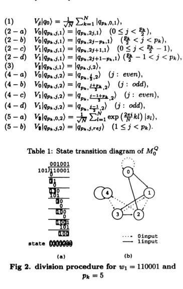
We give acomplete
state
transition diagram of
$M_{0}^{Q}$
in
Table
1,
where
$V_{\sigma}|Q\rangle$
$=\alpha_{1}|Q_{1}\rangle$
$+\cdots+\alpha:|Q:\rangle$
$+\cdots+$
$\alpha_{m}|Q_{m}\rangle$
means
that if
$M_{0}^{Q}$
reads symbol
$\sigma$in
state
$Q$
, it
moves
to
each state
$Q_{\dot{1}}$with amplitude
$\alpha:(|\alpha_{1}|^{2}+\cdots+$
$|\alpha_{m}|^{2}=1)$
.
When reading
$t$
of the input string
$fw_{1}\# w_{2}$
,
$M_{0}^{Q}$
splits
into
$N$
submachines
(denoted
by
$M_{1:}$
in Fig
1with equal
$\mathrm{s}\mathrm{y}\mathrm{m}^{j}\mathrm{b}^{1}\mathrm{o}1q_{\mathrm{P}2},\cdot \mathrm{l}\mathrm{i}\mathrm{t}\mathrm{g}\mathrm{o}\mathrm{a}\mathrm{e}\mathrm{t}\mathrm{o}\mathrm{s}\mathrm{t}\mathrm{a}\mathrm{t}\mathrm{e}\mathrm{l}.\mathrm{B}\mathrm{y}\mathrm{r}\mathrm{e}\mathrm{a}\mathrm{d}\mathrm{i}\mathrm{n}\mathrm{g}\mathrm{t}\mathrm{h}\mathrm{e}\mathrm{s}\mathrm{e}\mathrm{c}\mathrm{o}\mathrm{n}\mathrm{d}\mathrm{s}\mathrm{y}\mathrm{m}- \mathrm{T}\mathrm{h}\mathrm{e}\mathrm{s}\mathrm{t}\mathrm{a}\mathrm{r}\mathrm{t}\mathrm{i}\mathrm{n}\mathrm{g}\mathrm{s}\mathrm{t}\mathrm{a}\mathrm{t}\mathrm{e}\mathrm{i}\mathrm{s}0\mathrm{a}\mathrm{n}\mathrm{d}\mathrm{b}\mathrm{y}\mathrm{r}\mathrm{e}\mathrm{a}\mathrm{d}\mathrm{i}\mathrm{n}\mathrm{g}\mathrm{t}\mathrm{h}\mathrm{e}\mathrm{f}\mathrm{f}\mathrm{i}\mathrm{r}\mathrm{s}\mathrm{t}$
bol 1, it
goes to state 3
$(=11)$
.
Now reading 0, it
goes
$\mathrm{t}\mathrm{o}\mathrm{s}\mathrm{t}\mathrm{a}\mathrm{t}\mathrm{e}\mathrm{l}\mathrm{s}\mathrm{i}\mathrm{n}\mathrm{c}\mathrm{e}\mathrm{l}\mathrm{l}0\mathrm{r}\mathrm{e}\mathrm{a}\mathrm{d}\mathrm{i}\mathrm{n}\mathrm{g}\mathrm{t}\mathrm{t}\mathrm{h}\mathrm{e}\mathrm{l}\mathrm{a}8\mathrm{t}\mathrm{s}\mathrm{y}\mathrm{m}$$\mathrm{b}\mathrm{o}1=$$1\mathrm{m}\mathrm{o}\mathrm{d} 101\mathrm{a}\mathrm{n}\mathrm{d}M_{0}\mathrm{e}\mathrm{n}\mathrm{d}b\cdot \mathrm{T}\mathrm{h}\mathrm{s}\mathrm{u}\mathrm{p}\mathrm{i}\mathrm{n}\mathrm{s}\mathrm{t}\mathrm{a}\mathrm{t}\mathrm{e}4.\mathrm{I}\mathrm{t}\mathrm{i}\mathrm{s}\mathrm{c}\mathrm{o}\mathrm{n}\mathrm{t}\mathrm{i}\mathrm{n}\mathrm{u}\mathrm{e}\mathrm{s}\mathrm{u}\mathrm{n}\mathrm{t}\mathrm{i}\mathrm{l}$
should
be noted that these state transitions
are
reversible:
For example,
if the machine reaches
state 2
$(=10)$
from
some
state
$Q$
by reading 0, then
$Q$
must
be
state
1since
$Q$
cannot
be
greater than 2.
(Reason:
If
$Q$
is greater than
2, it
means
that the
quotient
will
be
1after reading
anew
$\mathrm{s}\mathrm{i}\mathrm{g}\mathrm{n}\mathrm{i}\mathrm{f}\mathrm{f}\mathrm{i}\mathrm{c}\mathrm{a}\mathrm{n}\mathrm{t}\mathrm{b}\mathrm{i}\mathrm{t}\mathrm{o}\mathrm{f}\mathrm{t}\mathrm{t}\mathrm{s}\mathrm{y}\mathrm{m}\mathrm{b}\mathrm{o}\mathrm{l}.\mathrm{S}\mathrm{i}\mathrm{n}\mathrm{c}\mathrm{e}M^{Q}\mathrm{e}\mathrm{r}\mathrm{a}\mathrm{e}\mathrm{i}\mathrm{d}\mathrm{u}\mathrm{e}\mathrm{w}\mathrm{h}\mathrm{e}\mathrm{n}\mathrm{d}\mathrm{i}\mathrm{v}\mathrm{i}\mathrm{d}\mathrm{e}\mathrm{d}\mathrm{b}\mathrm{y}5\mathrm{m}\mathrm{r}\mathrm{e}\mathrm{a}\mathrm{d}\mathrm{s}0\mathrm{a}\epsilon \mathrm{t}\mathrm{h}\mathrm{e}\mathrm{n}\mathrm{e}\mathrm{w}\mathrm{s}\mathrm{y}\mathrm{m}\mathrm{b}\mathrm{o}\mathrm{l}$
,
$\mathrm{t}\mathrm{h}\mathrm{e}\mathrm{l}\mathrm{e}\mathrm{a}\mathrm{s}\mathrm{t}\mathrm{u}\epsilon \mathrm{t}\mathrm{b}\mathrm{e}\mathrm{l}$,
which excludes state 2as
its
next
state.)
Hence
the
quo
then
must
have
been
0, and
so
the
previous
state must
be
1.
(Note
that this argument holds because
we
excluded
two
from
$pk$
which is only
one
even
prime.)
Thus,
if
$w_{1}\mathrm{m}\mathrm{o}\mathrm{d} pk$
$=j_{k}$
, then
$M_{0}^{Q}$
is in superposition
$\frac{1}{\tau}\sum_{k=1}^{N}N|q_{\mathrm{p}_{k},f_{k},1})$
after
$M_{0}^{Q}$
read
$w_{1}$
.
Then
$M_{0}^{Q}$
reads
$\#$and this
superposition is
“shiRed” to
$\frac{1}{\sqrt{N}}\sum_{k=1}^{N}|q_{\mathrm{p}_{k},j_{k},2}\rangle$
,
where
$M_{0}^{Q}$
checks
$1\mathrm{f}w_{2}^{R}\mathrm{m}\mathrm{o}\mathrm{d} pk$is also
$j_{k}$
by using
tran-sition
$(4-a)$
to
$(4-d)$
in
Table 1. This
job
can
be
done
by completely
reversing
the previous procedure
of
dividing
$w_{1}$
by
$p_{k}$
.
Actually, the
state
transitions
are
obtained
by
simply reversing
the directions of
previous
state diagrams.
Since
previous
transitions
are
reversible,
new
transitions
are
also reversible.
Now
one can see
that the
$k$
-th
sub
machine
$M_{2k}$
is in
state
$q_{\mathrm{p}_{k},0,2}$iff
the
two
residues
are
the
same.
Finally by
reading
$,
Fourier transform is carried out
only
from these zer0-residue
states
$q_{p_{k},0,2}$
to
$s\iota$.
Other
$\mathrm{S}\mathrm{t}\mathrm{a}\mathrm{t}\mathrm{e}\mathrm{s}q_{p_{k},j,2}\mathrm{r}\mathrm{e}\mathrm{S}\mathrm{i}\mathrm{d}\mathrm{u}\mathrm{e}\mathrm{s}\mathrm{a}\mathrm{r}\mathrm{e}\mathrm{t}\mathrm{t}_{\mathrm{e}\mathrm{s}\mathrm{a}\mathrm{m}\mathrm{e}\mathrm{i}\mathrm{n}\mathrm{o}\mathrm{n}1\mathrm{y}t\mathrm{s}\mathrm{u}\mathrm{b}\mathrm{m}\mathrm{a}\mathrm{c}\mathrm{h}\mathrm{i}\mathrm{n}\mathrm{e}\mathrm{s}^{k}\mathrm{o}\acute{\mathrm{u}}\mathrm{t}\mathrm{o}\mathrm{f}\mathrm{t}\mathrm{h}\mathrm{e}k}^{j\neq 0)\mathrm{g}\mathrm{o}\mathrm{t}\mathrm{o}\mathrm{r}\mathrm{e}\mathrm{j}\mathrm{e}\mathrm{c}\mathrm{t}\mathrm{i}\mathrm{n}\mathrm{g}\mathrm{s}\mathrm{t}\mathrm{a}\mathrm{t}\mathrm{e}\mathrm{s}q_{p,jrej}.\mathrm{I}\mathrm{f}\mathrm{t}\mathrm{h}\mathrm{e}}$
ones, the amplitude of
$s_{N}$
is given
as
$\frac{1}{N}\sum_{|t|}\sum_{\mathrm{t}=1}^{N}\exp(\frac{2\pi i}{N}kl)|s_{\mathrm{t}}\rangle$
$= \frac{t}{N}|s_{N}\rangle+\frac{1}{N}\sum_{|t|}\sum_{\mathrm{t}=1}^{N-1}\exp(\frac{2\pi i}{N}kl)|s_{l}\rangle$
,
which is equal to
$t/N$
.
Thus the probability of
acceptance
is
$(_{F}^{t})^{2}$
.
If
the input
string
is in
$L_{0}$
, then this probability
becomes
1.
Otherwise,
it is at
most
$(N_{0}/N)^{2}$
by Lemma
2. The number of
states
in
$M_{0}^{Q}$
is given
as
$1+2k \sum_{=1}^{N}p_{k}+\sum_{k=1}^{N}(p_{k}-1)+N$
$=1+3 \sum_{k=1}^{N}p_{k}\leq 1+3\cdot$
$N\cdot$
$p_{N}=O(N^{2}\log N)$
,
which completes the proof.
$\blacksquare$(1)
$V_{\beta}|q \mathrm{o}\rangle=\frac{1}{\sqrt{N}}\sum_{k=1}^{N}|q_{p_{k},0,1}\rangle$
,
$(2-a)$
$V_{0}|q_{\mathrm{p}_{k},j,1})=|q_{p_{k},2j,1})$
$(0\leq j<\epsilon_{2}\iota_{)}$
,
$(2-b)$
$V_{0}|q_{\mathrm{p}_{k\prime}j,1}\rangle=|q_{\mathrm{p}_{k\prime}2j-\mathrm{p}_{k}.1}\rangle$
$(_{2}^{\mathrm{h}}<i<p_{k})$
,
$(2-c)$
$V_{1}|q_{\mathrm{p}_{k},j,1}\rangle=|q_{\mathrm{p}_{k},2j+1,1}\rangle$
$(0\leq j<\epsilon_{2}\mathrm{h}-1)$
,
$(2-d)$
$V_{1}|q_{\mathrm{p}_{k},j,1}\rangle=|q_{p_{k},2j+1-\mathrm{p}_{k},1})(_{2}^{\mathrm{h}}-1<j<p_{k})$
,
(3)
$V_{\mathrm{t}}|q_{\mathrm{p}_{k},j,1}\rangle=|q_{p_{k\prime}j.2}\rangle$
,
$(4-a)$
$V_{0}|q_{p_{k},j,2}\rangle=|q_{\mathrm{P}k},:,2)$
(
$j$
:
even),
$(4-b)$
$V_{0}|q_{\mathrm{p}_{k},j,2})=|q_{\mathrm{P}k},J++,2\rangle$
(
$j$
:
odd),
$(4-c)$
$V_{1}|q_{p_{k},j,2}\rangle=|q_{\mathrm{P}k},\underline{g-}1+\neq 1,2\rangle$
(
$j$
:
eaten),
$(4-d)$
$V_{1}|q_{\mathrm{p}_{k}.j,2}\rangle=|q_{\mathrm{p}_{k},arrow^{-1}.2}\rangle$
(
$j$
:
odd)
,
$(5-a)$
$V_{1}|q_{p_{k},0,2})= \tau_{N}^{1}\sum_{\mathrm{t}=1}^{N}\exp(_{\mathrm{T}^{\dot{1}}}^{2\pi}kl)|s_{\mathrm{t}\rangle}$
,
$(5-b)$
$V_{1}|q_{p_{k}.j,2}\rangle=|q_{p_{k\prime}j,\tau \mathrm{e}f}\rangle$
$(1\leq j<p_{k})$
.
$\mathrm{t}\mathrm{a}\mathrm{I}$
$1\mathrm{b}\mathfrak{l}$
Fig
2. division procedure for
$w_{1}=110001$
and
$p_{k}=5$
Let
us
consider the pfa whose
state
transition is exactly
the
same
as
$M_{0}^{Q}$
of
$f(N)$
states
excepting that
the state
transitions from
$\mathrm{q}\mathrm{P}\mathrm{k},0,2$to
$s\iota$for
Fourier transform
are
re-placed by simple
(deterministic) transitions from
$q_{p_{k},0,2}$
to
$s_{N}$
.
We call such apfa emulates the
$\mathrm{q}\mathrm{f}\mathrm{a}$.
Suppose that
$M^{P}$
emulates
$M^{Q}$
.
Then the size of
$M^{P}$
is
almost the
same as
that of
$M^{Q}$
,
i.e., it is also
$\Theta(f(N))$
if
the
latter
is
$f(N)$
,
since
the
Fourier transform does not make much
difference
in
the number of
states.
$\mathrm{a}\mathrm{c}\mathrm{c}\mathrm{e}\mathrm{p}\mathrm{t}\mathrm{s}\mathrm{s}\mathrm{t}\mathrm{r}\mathrm{i}\mathrm{n}\mathrm{g}\mathrm{s}\mathrm{i}\mathrm{n}L_{0}\mathrm{w}\mathrm{i}\mathrm{t}\mathrm{h}\mathrm{p}\mathrm{r}\mathrm{o}\mathrm{t}\mathrm{a}\mathrm{b}\mathrm{i}1\mathrm{i}\mathrm{t}\mathrm{y}\mathrm{o}\mathrm{n}\mathrm{e}\mathrm{a}\mathrm{n}\mathrm{d}\mathrm{t}\mathrm{h}\mathrm{o}\mathrm{s}\mathrm{e}\mathrm{n}\mathrm{o}\mathrm{t}\mathrm{L}\mathrm{e}\mathrm{m}\mathrm{m}\mathrm{a}4.\mathrm{S}\mathrm{u}\mathrm{p}\mathrm{p}\mathrm{o}\mathrm{s}\mathrm{e}\mathrm{t}\mathrm{h}\mathrm{a}\mathrm{t}M^{P}\mathrm{e}\mathrm{m}\mathrm{u}1\mathrm{a}\mathrm{t}\mathrm{e}\mathrm{s}M_{0}^{Q}.\mathrm{T}\mathrm{h}\mathrm{e}\mathrm{n}M_{0}^{P}$
in
$L_{0}$
with
probability
$N_{0}/N$
.
Let
us
set,
for example,
$N=N_{0}\sqrt{n}$
.
Then the
error-rate
of
$M_{0}^{Q}$
is
$(N_{0}/N)^{2}= \frac{1}{n}$
and its size is
$o(n^{3}/\log n)$
.
To
achieve the
same
error-rate by
a
$\mathrm{p}\mathrm{f}\mathrm{a}$,
we
have to set
$N=N_{0}n$
,
which needs
$O(n^{4}/\log n)$
states.
Remark.
Suppose that
we
have
once
designed
aspecific
$\mathrm{q}\mathrm{f}\mathrm{a}M_{0}^{Q}$
(similar for
$M_{0}^{P}$
).
Then it
can
work for
inputs of
any length
or
it
does not reject the input only for the
reason
that its length is not
$2n+1$
.
The above calculation
of the
acceptance
and rejection rates is only true when
our
input is
restricted to
strings
$\subseteq\{0,1\}^{n}\#\{0,1\}\mathrm{n}$
.
Now
we
shall design
aqfa
$M_{1}^{Q}$
which
recognizes
the
second
language
$L_{1}(n)$
.
$N_{0}’$
also denotes the number
$s$
in
Lemma 1but for
$x$
and
$y$
of
length
$2n$
.
Lemma 5. There exists
a
$\mathrm{q}\mathrm{f}\mathrm{a}M_{1}^{Q}$which
accepts
strings
in
$L_{1}$
with probability
$1-( \frac{N}{N}\Delta 1)^{2}+(\frac{N}{N}\mathrm{n}_{1})^{4}$
and strings not
in
$L_{1}$
with
at
most
$( \frac{N}{N}\mathrm{n}_{1})^{2}+(\frac{N}{N}\acute{\alpha}2)^{2}\cdot(1-\frac{N}{N}\Delta 1)^{2}\cdot(1+\frac{N}{N}\mathrm{n}_{1})^{2}$
.
$M^{Q}\mathrm{h}\mathrm{a}\mathrm{s}\Theta((N_{1}N_{2})^{2}1\mathrm{o}\mathrm{b}\mathrm{r}\mathrm{o}\mathrm{o}\mathrm{f}.\mathrm{A}\mathrm{g}\mathrm{a}\mathrm{i}\mathrm{n}\mathrm{a}\mathrm{c}\mathrm{o}\mathrm{g}N_{1}\cdot\log N_{2})\mathrm{s}\mathrm{t}\mathrm{a}\mathrm{t}\mathrm{e}\mathrm{s}\mathrm{m}\mathrm{p}1\mathrm{e}\mathrm{t}\mathrm{e}\mathrm{s}\mathrm{t}\mathrm{a}\mathrm{t}\mathrm{e}\mathrm{t}\mathrm{r}\mathrm{a}\mathrm{n}\mathrm{s}\mathrm{i}\mathrm{t}.\mathrm{i}\mathrm{o}\mathrm{n}$
diagram is
shown in Table 2, where accepting
states
are
$s_{N_{1},0,p\iota,f}$
such that
$0\leq f<pl-1$
and
$t_{N_{1}}$
.
Rejecting states
are
$q_{p_{k},e,pf,rej},$
,such
$\mathrm{t}-\mathrm{h}\mathrm{a}\mathrm{t}e\neq 0$or
$f\neq 0$
,
$0<e\leq p_{k}-1$
,
$0\leq f\leq pl$
$-1$
,
$t_{p_{k},0,y}$
such that
$1\leq y\leq\overline{N}_{2}-1$
, and
$t_{z}$such that
$1\leq z\leq N_{1}-1$
.
All other states
are
non-halting.
$M_{1}^{Q}$
checks whether
$w_{1}=w_{2}^{R}$
using
$N_{1}$
primes
and also
whether
$(w_{1}w_{2})=(w_{3}w_{4})^{R}$
using
$N_{2}$
primes.
Note that
those
jobs
have to be done at the
same
using
composite
automata while reading
$w_{1}\# w_{2}$
.
Hence
$M_{1}^{Q}$
first
splits
into
$N_{1}\cdot$
$N_{2}$
submachines, each of which is denoted by
At(k,
$l$
),
$1\leq k\leq N_{1},1\leq l\leq N2$
.
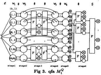
As shown
in
Fig 3,
$M(k, l)$
has six stages, from stage 1thorough stage 6. It might be
convenient to think that each state of
$M(k, l)$
be
apair
of state
$(q_{L}, q_{R})$
and to think
$M(k, l)$
be
acomposite
of
$M_{L}$
and
$M_{R}$
.
In stages 1and 2,
$M_{L}$
has asimilar state
transitions
to those of Table 1for checking
$w_{1}\neq w_{2}^{R}$
.
$M_{R}$
has also similar transitions but only for the first
part
of
it,
i.e.,
to
compute WIW2
$\mathrm{m}\mathrm{o}\mathrm{d} \mathrm{p}\mathrm{i}$.
This
portion
of transitions
are
given in
(2)
to
(4)
of Table
2.
$\#$
,
carries
out
the
Fourier transform
exactly
as
$M_{0}^{Q}$
(see
$\int_{\mathrm{e}\mathrm{x}\mathrm{e}\mathrm{c}\mathrm{u}\mathrm{t}\mathrm{e}\mathrm{I}\mathrm{n}\mathrm{v}\mathrm{e}\mathrm{r}\mathrm{s}\mathrm{e}\mathrm{F}\mathrm{o}\mathrm{u}\mathrm{r}\mathrm{i}\mathrm{e}\mathrm{r}\mathrm{t}\mathrm{r}\mathrm{a}\mathrm{n}\mathrm{s}\mathrm{f}\mathrm{o}\mathrm{r}\mathrm{m}\mathrm{f}\mathrm{f}\mathrm{o}\mathrm{m}\mathrm{s}\mathrm{t}\mathrm{a}\mathrm{t}\mathrm{e}8S_{m,0,\mathrm{p}\iota,f}}^{5-a)\mathrm{i}\mathrm{n}\mathrm{T}\mathrm{a}\mathrm{b}1\mathrm{e}2).\mathrm{A}\mathrm{f}\mathrm{f}\mathrm{i}\mathrm{e}\mathrm{r}\mathrm{t}\mathrm{h}\mathrm{a}\mathrm{t}M_{L},\mathrm{r}\mathrm{e}\mathrm{a}\mathrm{d}\mathrm{i}\mathrm{n}\mathrm{g}\mathrm{t}\mathrm{h}\mathrm{e}\mathrm{s}\mathrm{e}\mathrm{c}\mathrm{o}\mathrm{n}\mathrm{d}}$
,
$(1 \leq m\leq N_{1}-1)$
,
i.e.,
ffom the states after the first
Fourier transform excepting the accepting states, which is
shown
in
$(6-a)$
of
Table 2.
In
this stage,
$M_{R}$
does
noth-ing; it just
shifts
the
state
information about
$(w_{1}w_{2})$
mod
$p\mathrm{t}4_{\mathrm{t}\mathrm{a}\mathrm{g}\mathrm{e}\mathrm{s}4\mathrm{a}\mathrm{n}\mathrm{d}5\mathrm{a}\mathrm{r}\mathrm{e}\mathrm{f}\mathrm{o}\mathrm{r}\mathrm{t}\mathrm{h}\mathrm{e}\mathrm{c}\mathrm{o}\mathrm{m}\mathrm{p}1\mathrm{e}\mathrm{t}\mathrm{e}}^{\mathrm{b}\mathrm{u}\mathrm{t}\mathrm{o}\mathrm{n}1\mathrm{y}\mathrm{w}\mathrm{h}\mathrm{e}\mathrm{n}w_{1}\neq w_{2}^{R})\mathrm{t}\mathrm{o}\mathrm{s}\mathrm{t}\mathrm{a}\mathrm{g}\mathrm{e}4}$
.reverse
operation
of stages 2and 1. By doing this, the amplitudes for state
$qL$
, which
were
once
in turmoil after stage 2,
are
reorga-nized and gathered in
specific
states, namely
$q_{p_{k},0,p\iota,0,4}$
if
$(w_{1}w_{2})=(w_{3}w_{4})^{R}$
.
Therefore,
what
we
do is to gather
$\mathrm{f}_{\mathrm{o}\mathrm{r}\mathrm{m}\mathrm{r}\mathrm{e}\mathrm{a}\mathrm{d}\mathrm{i}\mathrm{n}\mathrm{g}\#.0^{\mathrm{P}\mathrm{P}1}}\mathrm{t}\mathrm{h}\mathrm{e}\mathrm{a}\mathrm{m}\mathrm{p}1\mathrm{i}\mathrm{t}\mathrm{u}\mathrm{d}\mathrm{e}\mathrm{o}_{\mathrm{N}\mathrm{w}^{k}\mathrm{r}\mathrm{e}\mathrm{a}\mathrm{d}\mathrm{i}^{4}\mathrm{g}\mathrm{t}\mathrm{h}\mathrm{e}\mathrm{r}\mathrm{i}\mathrm{g}^{0}\mathrm{h}_{\mathrm{t}\mathrm{m}\mathrm{o}\mathrm{s}\mathrm{t}\mathrm{s}\mathrm{y}\mathrm{m}\mathrm{b}\mathrm{o}1,\mathrm{w}\mathrm{e}\mathrm{d}\mathrm{o}}^{N_{2}}}\mathrm{f}q,0,0_{\mathrm{I}1},\mathrm{t}\mathrm{o}t_{\mathrm{P}k},\mathrm{b}\mathrm{y}\mathrm{F}\mathrm{o}\mathrm{u}\mathrm{r}\mathrm{i}\mathrm{e}\mathrm{r}\mathrm{t}\mathrm{r}\mathrm{a}\mathrm{n}\mathrm{s}-$
another Fourier transform, which gathers the amplitudes
$\mathrm{o}\mathrm{f},\mathrm{t}\mathrm{o}t_{N_{1}}\oint_{\mathrm{h}^{k}\mathrm{e}\mathrm{a}\mathrm{n}\mathrm{a}1\mathrm{y}\mathrm{s}\mathrm{i}\mathrm{s}\mathrm{o}\mathrm{f}}^{t0,N_{2}}$.error
probability is alittle bit
compli-cated. The basic idea is
as
follows: When
$w_{1}\neq w_{2}^{R}$
,
a
small
amplitude,
$\frac{1}{\sqrt{2}}\frac{N}{N}A1$is
“taken” by each of the
$N_{2}$
ac-cepting states in stage 3. This is basically the
same as
$M_{0}^{Q}$
since its probability of observation is
$\sum_{\mathrm{t}=1}^{N_{2}}(\frac{1}{\sqrt{2}}\cdot \mathrm{r}N)^{2}N_{1}=$
$(N\neq_{1})^{2}$
.
So, the
problem
is
how much of the remaining
am-plitudes
distributed
on
other
states
in
this stage
can
be
retrieved
in
the final accepting state
$t_{N_{1}}$
when
(WIW2)
$=$
$(w_{3}w_{4})^{R}$
.
If
we
could retrieve
100%,
then the
accept-ing
probability at state
$t_{N_{1}}$
when
(WIW2)
$=(w_{3}w_{4})^{R}$
is
$1-( \frac{N}{N}\Delta)^{2}1^{\cdot}$
Unfortunately,
we
cannot
do that but the loss
is
very small and
our
accepting probability at state
$t_{N_{1}}$
is
$(1-( \frac{N_{0}}{N_{1}})^{2})^{2}=1-2(\frac{N_{0}}{N_{1}})^{2}+(\frac{N_{0}}{N_{1}})^{4}$
which turns out to be enough for
our
purpose.
SS
Suppose that
we
set
$N_{1}=N_{0}\sqrt{n}$
, and
$N_{2}=dN_{0}’$
.
Then
$\frac{N}{N}\mathrm{n}_{1}=T^{1}n$
and
$\frac{N}{N}\mathrm{A}2’\leq\frac{1}{2}$if
we
select asufficiently large
constant
$d$
.
Namely,
$M_{1}^{Q}$
accepts
strings in
$L_{1}$
with
prob-ability 1
$- \frac{1}{n}+\overline{n}^{\mathrm{V}}1$and those not in
$L_{1}$
with probability
at most
$\frac{1}{4}+\frac{1}{2n}+\overline{n}^{T}1$
.
The number of states is
$\Theta(_{1\hat{\mathrm{o}\mathrm{g}n}}^{n^{5}})$.
The probability
distribution
on
acceptance and rejection
in
each state is illustrated in Fig 4.
$\mathrm{s}\mathrm{c}\mathrm{a}\mathfrak{g}\mathrm{e}\mathrm{l}$
stage2
$*\mathrm{t}*\mathrm{g}\mathrm{e}3$ $.\mathrm{t}\mathrm{p}\cdot\ell*\mathrm{t}*\mathfrak{g}\cdot 5$ $.\mathrm{t}\cdot \mathfrak{g}\cdot 6$Fig 3.
$\mathrm{q}\mathrm{f}\mathrm{a}M_{1}^{Q}$Now
we
go to stage 3. Here
$M_{L}$
, reading the first
Fig 4. probability distribution when
$N_{1}=\mathrm{N}\mathrm{o}$
$\mathrm{n}$,
$N_{2}=dN_{0}’$
Let
us
consider
$\mathrm{p}\mathrm{f}\mathrm{a}M_{1}^{P}$which recognizes
$L_{1}(n)$
.
The
state
transition of
$M_{1}^{P}$
is the
same
as
that of
$M_{1}^{Q}$
except
Fourier transform and
Inverse Fourier
transform only
$M_{1}^{Q}$
performs.
If string
$x$
satisfies
$w_{1}\neq w_{2}^{R}$
,
then
$M_{1}^{P}$
accepts
$x$
with at most probability
$\frac{N}{N}\mathrm{n}_{1}$after reading
$w_{1}\# w_{2}$
.
It
should be noted that
$M_{1}^{Q}$
accepts
such
astring
with at
most
probability
$( \frac{N}{N}A)^{2}1$
after
reading
$w_{1}\# w_{2}$
.
Lemma
6.
Suppose
that
$M_{1}^{P}$
emulates
$M_{1}^{Q}$
.
Then
$M_{1}^{P}$
accepts strings in
$L_{1}$
with probability 1and those
not
in
$L_{1}$
with probability
at
most
$\frac{N}{N}\mathfrak{g}1+(1-N\mathrm{n})\overline{\overline{N}}_{1}$.
$\frac{N}{N}\acute{\mathrm{A}}2^{\cdot}$The number of
states
is approximately the same, i.e.,
$\Theta((N_{1}N_{2})^{2}\log N_{1}\log N_{2})$
.
(Proof
is
omitted.)
If
we
set
$N_{1}=N_{0}n$
and
$N_{2}=dN_{0}’$
, then strings such
that
$w_{1}\neq w_{2}^{R}$
are
accepted with probability at
most
$\frac{1}{n}$after reading
$w_{1}\# w_{2}$
.
Thus this probability is the
same as
the qfa
such that
$N_{1}=N_{0}\sqrt{n}$
and
$N_{2}=dN_{0}’$
,
but
number
of states of this pfa is
$\Omega(_{1\mathrm{o}\mathrm{g}\overline{n}}^{n^{0}}\neg)$.
Now
we
are
ready
to give
our
main theorem:
Theorem 1. For
any
integer
$c$
,
there is
a
$\mathrm{q}\mathrm{f}\mathrm{a}M^{Q}$such
that
$M^{Q}\mathrm{r}$
cognizes
$L(n, n^{\mathrm{c}})$
and the number of states in
$M^{Q}$
is
0
$(_{1\mathrm{o}\mathrm{g}}^{n^{\epsilon+}} \neg\frac{4}{n})$.
Proof. The
construction
of
$M^{Q}$
is
easy:
We just
add
a
new
deterministic transition from
the last accepting state
in stage 6of
$M_{1}^{Q}$
to its
initial
state
by
$\#$,
by which
we
can
manage
iteration. Also,
we
need
some
small changes
to manage
the
very
end of the string: Formally speaking,
transition
(11)
in
Table 2is
modified into
$V_{\#}|t_{\mathrm{p}_{k},0,N_{2}} \rangle=\frac{1}{\sqrt{N_{1}}}\sum_{z=1}^{N_{1}}\exp(\frac{2\pi i}{N_{2}}kz)|t_{t})$
,
$t_{N_{1}}\mathrm{i}\epsilon$
now
not
an
accepting
state but anon-halting
state
and two
new
transitions
$(10-c)$
$V.|q_{\mathrm{P}k,\mathrm{e},p\iota,f,4}\rangle=|q_{p_{k}.\mathrm{e},p\iota,f,r\mathrm{e}j}\rangle$
(12)
$V_{t}|t_{N_{1}})=|q_{1})$
are
added.
We
set
$N_{1}=2N_{0}n^{\mathrm{c}/2}$
and
$N_{2}=dN_{0}’$
.
Then
$N_{0}/N_{1}=$
$\frac{1}{2n^{\mathrm{e}/2}}$and
$N_{0}’/N_{2}< \frac{1}{2}$
if
we
select
asufficiently
large
con-stant
as
$d$
.
Suppose that
$M^{Q}$
has
not
stopped
yet
and
is
now
reading the
$i$
-th
block
$w:1\# w_{\dot{1}2}\#\# w_{\dot{|}s}\# w_{\dot{1}4}$
.
Then,
we
can
conclude the following by Lemma
5:
(i)
If
$w:1=w_{\dot{1}2}^{R}$
,
then
$M^{Q}$
accepts the input with probability
one.
(ii)
If
$(w:1w_{i2})=(w_{i3}w_{\dot{1}4})^{R}$
,
then
$(:i-a)M^{Q}$
als0
accepts
the
input
with probability
$1/4n^{\mathrm{c}}$
and
$(ii-b)$
rejects
the
input
with
$\frac{1}{4n^{\mathrm{c}}}-\overline{1}\infty^{1}\Gamma \mathrm{e}$and
$(|.:-c)$
goes
back to the initial
state
with 1(ii) If
$(w_{11}w_{\dot{1}2})\neq(w_{\dot{1}3}w_{\dot{1}4})^{R}$
,
then
$(\mathrm{i}\mathrm{i}-a)M^{Q}$
accepts
the input with
$\frac{1}{4n^{e}}$,
$(\mathrm{i}\mathrm{i})-b)$
rejects
it
with
$I- \frac{1}{8n^{e}}-16\neg n31$
$\overline{e}$and
$(\mathrm{i}\mathrm{i}-c)$
goes back to
the
ini-tial
state
with
1
$- \frac{1}{8n^{\mathrm{c}}}+\neg 1\epsilon_{\hslash}^{1}\overline{\epsilon}$.
The number of
state
is
$o\mathrm{R}^{n^{\mathrm{c}+}}4\mathrm{A}_{\mathrm{t}\mathrm{h}\mathrm{a}\mathrm{t}\mathrm{t}\dot{\mathrm{h}}\mathrm{e}}^{1\mathrm{o}\mathrm{g}^{2}n)}$
number of iteration is
$n^{\mathrm{c}}$and
suppose
is
at most
$\frac{1}{4n^{e}}$per
iteration,
and
so
the probability that
$(:i-b)$
happens in
some
iteration is
at most
$n^{\mathrm{c}}\cdot$$\frac{1}{4n^{c}}=$
$\not\supset 1$
.
Therefore
the probability
that
$x$
is finally accepted is
well
larger than 1/2.
Suppose
conversely that
$x$
is
not
in
$L(n,n^{\mathrm{c}})$
.
Then
the
probability
that
$(ii-a)$
happens in
some
iteration is
the
same as
above and is at
most
$\frac{1}{4}$.
If
$M^{Q}$
do
$\mathrm{s}$not
meet ablock such
that
$(w:1w:2)\neq(w_{\dot{1}3}w_{\dot{l}4})^{R}$
until the end, then the accepting probability is
at most
this
1/4.
If
$M^{Q}$
do
$\mathrm{s}$meet such
ablock in
some
iteration,
it
rejects
$x$
with
probability
at
least
$(1 - \frac{1}{4})(\frac{3}{4}-\frac{1}{8n^{c}}$
-$\neg 16ne1)$
which is again well above 1/2. Thus
$M^{Q}$
recognizes
$L(n,n^{\mathrm{c}})$
.
$\blacksquare$Theorem
2. Suppose that
$M^{P}$
which
emulates
$M^{Q}$
recognizes
$L(n, n^{\mathrm{c}})$
.
Then the number of states
of
$M^{P}$
is
$\Omega(n^{2\mathrm{c}+4}/\log^{2}n)$
.
Proof.
$M^{P}$
is
constructed by applying asimilar
modi-fication
as
above
to
$M_{1}^{P}$
.
Then it
turns
out
from Lemma
6that if
we
set
$N_{1}= \frac{1}{a}N_{0}n^{\mathrm{c}}$
,
$N_{2}=dN_{0}’$
then the number
$\mathrm{t}\mathrm{h}\mathrm{e}\mathrm{i}\mathrm{n}\mathrm{p}\mathrm{u}\mathrm{t}\mathrm{o}\mathrm{f}\mathrm{s}\mathrm{t}\mathrm{a}\mathrm{t}\mathrm{e}\mathrm{s}$$\mathrm{i}\mathrm{n}M^{P}\mathrm{i}\mathrm{s}\Omega(n^{2\mathrm{c}+4}/1\mathrm{o}\mathrm{g}^{2}n)x\mathrm{i}\mathrm{n}\mathrm{c}1\mathrm{u}\mathrm{d}\mathrm{e}\mathrm{s}\mathrm{a}1\mathrm{o}\mathrm{n}\mathrm{g}\mathrm{r}\mathrm{e}\mathrm{p}\mathrm{e}\mathrm{t}\mathrm{i}\mathrm{t}\mathrm{i}\mathrm{o}.\mathrm{n}\mathrm{o}\mathrm{f}\mathrm{b}1_{\mathrm{o}\mathrm{C}}\mathrm{k}\mathrm{s}\mathrm{s}\mathrm{u}\mathrm{c}\mathrm{h}\mathrm{t}\mathrm{h}\mathrm{a}\mathrm{t}\mathrm{N}\mathrm{o}\mathrm{w}\mathrm{s}\mathrm{u}\mathrm{p}\mathrm{p}\mathrm{o}\mathrm{s}\mathrm{e}\mathrm{t}\mathrm{h}\mathrm{a}\mathrm{t}$
$(w:1w_{\dot{1}2})=(w_{\dot{1}3}w_{\dot{1}4})^{R}$
.
Then
$x$
is accepted
in
each
itera-tion with probability
$a/n^{\mathrm{c}}$.
Therefore the
probability that
this happens in the first
$k$
iterations is
$\sum_{\dot{l}=1}^{k}(1-\frac{a}{n^{\mathrm{c}}})^{x-1}\cdot\frac{a}{n^{\mathrm{c}}}=1-(1-\frac{a}{n^{\mathrm{c}}})^{k}$
Since
the number of repetitions
$(=k)$
can
be
as
large
as
$n^{\mathrm{c}}$
,
$\lim_{narrow\infty}(1-\frac{a}{n^{\mathrm{c}}})^{n^{e}}=\frac{1}{e^{a}}$
.
Thus if
we
select asufficiently large constant
$a$
, then
the
$\mathrm{C}\mathrm{a}\mathrm{n}\mathrm{n}\mathrm{o}\mathrm{t}\mathrm{r}\mathrm{e}\mathrm{c}\mathrm{o}\mathrm{g}\mathrm{n}\mathrm{i}\mathrm{z}\mathrm{e}L\mathrm{P}^{\mathrm{r}\mathrm{o}\mathrm{b}\mathrm{a}\mathrm{b}\mathrm{i}1\mathrm{i}\mathrm{t}\mathrm{y}\mathrm{o}\mathrm{f}\mathrm{a}\mathrm{c}\mathrm{c}\mathrm{e}}\xi_{n,n^{\mathrm{c}})\mathrm{o}\mathrm{b}\mathrm{v}\mathrm{i}\mathrm{o}\mathrm{u}\mathrm{s}1\mathrm{y},\mathrm{w}\mathrm{h}\mathrm{i}\mathrm{c}\mathrm{h}\mathrm{p}\mathrm{r}\mathrm{o}\mathrm{v}\mathrm{e}\mathrm{s}\mathrm{t}\mathrm{h}\mathrm{e}\mathrm{t}\mathrm{h}\underline{\mathrm{e}-}}^{\mathrm{t}\mathrm{a}\mathrm{n}\mathrm{c}\mathrm{e}\mathrm{c}\mathrm{a}\mathrm{n}\mathrm{b}\mathrm{e}\mathrm{a}1\mathrm{m}\mathrm{o}\mathrm{s}\mathrm{t}1.\mathrm{S}\mathrm{u}\mathrm{c}\mathrm{h}\mathrm{a}M^{P}}$