A Study on Stepwise Satisfaction Method of Constraints for Many Constrained Optimization Problem

全文

(1)Vol.2018-MPS-119 No.7 2018/7/30. IPSJ SIG Technical Report. A Study on Stepwise Satisfaction Method of Constraints for Many Constrained Optimization Problem Tomohiro Yoshikawa1,a). Kento Niwa1,b). Abstract: Due to the improvement of performance of computers, Genetic Algorithm is actively applied to actual en-. gineering problems. Most of engineering problems are constrained optimization problems which optimize objective functions under the conditions of many constraints. Penalty method is well-known as the optimizer for such constrained optimization problems. However, the benchmarks of constrained optimization problems have only small number of constraints. Thus, the effectiveness of penalty method has not been investigated in many constrained problems. In many constrained optimization problems, the penalty method has a risk that all constraints cannot be satisfied. This paper proposes the stepwise satisfaction method of constraints to satisfy many constraints. In the proposed method, the priority of constraints to be satisfied is defined based on the initial population. In the experiment, the performance of the proposed method and the penalty method was compared in two problems which have more than 50 constraints. Keywords: multi-constrained optimization problem, stepwise satisfaction method of constraints, difficulty of con-. straints, penalty method,. 1.. Recently, the diversification of user needs has advanced in various fields. In order to respond to this needs, it is necessary to produce small amount but various kinds of industrial products. However, the production of small amount and various kinds increases the development and production cost. Therefore, a system of supporting design is needed. Genetic Algorithm attracts attention for this request, and various engineering applications of Genetic Algorithm have been reported [1], [2], [3]. Most of engineering applications are multi-constrained optimization problems. A multi-constrained optimization problem optimizes the objective functions under some constraints, which often has many constraints. Penalty method [4], [5] is often applied to constrained optimization problems. Generally, the performance of these algorithms is investigated by applying to benchmark problems, CDTLZ [6] and CF [7] are the representative examples. However, it is pointed out that the number of constraints is too small in these problems [8] (Table 1) considering the actual engineering applications. For this reason, these methods do not take into account many constraints and treat all constraints concurrently. However, when the constraints in a problem have different difficulties to be satisfied, it tries to satisfy easier constraints first due to the characteristics of Genetic Algorithm. That may result in a local solution for the constraint satisfaction and all constraints may not be satisfied. To satisfy all constraints, it is necessary to define search priority for constraints. 1. a) b). Table 1: Benchmark of Constrained Optimization Problems. Introduction. Graduate School of Engineering, Nagoya University, Aichi 464–8603, Japan [email protected] [email protected]. ⓒ 2018 Information Processing Society of Japan. Problems C-DTLZ CF1-3 CF4-7 CF8-10. Number of objective functions Variable 2 2 3. Number of constraints 1 1 1 or 2 1. Thus we propose a stepwise satisfaction method of constraints in this paper. The proposed method focuses on the difficulty of constraints and define the search priority for constraints based on their priorities. The proposed method defines the difficulty of constraints based on the information of initial population. In the parent selection, individuals which satisfy more difficult constraints are given priority. We conducted experiments to show the effectiveness of the proposed method. In the experiments, the proposed method was applied to two problems and compared with the static penalty method [9]. The problems which employed in the experiments were MOPTA08 [10] and the simultaneous design optimization benchmark problem of multiple car structure using response surface method [11], which have more than 50 constraints.. 2.. Constrained Optimization Problems. Eq. (1) and (2) show the general definition of the constrained optimization problems. Minimize f (x). (1). subject to gi (x) ≥ 0 (i = 1, 2, ..., k). (2). x is a solution. f (x) is the objective function and gi (x) are the constraints. The amount of constraint violation v(x) and the total amount of constraint violation Ω(x) are defined by eq. (3) and (4). 1.

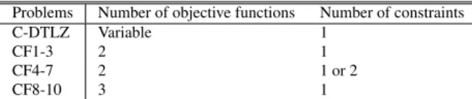
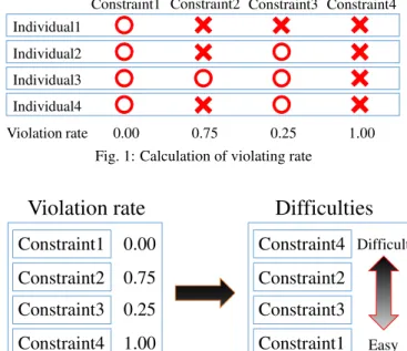
(2) Vol.2018-MPS-119 No.7 2018/7/30. IPSJ SIG Technical Report.     |gi (x)| vi (x) =    0 Ω(x) =. k ∑. i f (gi (x) < 0) (i = 1, 2, ..., k) otherwise. Constraint1 Constraint2 Constraint3 Constraint4. (3). Individual1 Individual2. vi (x). (4). Individual3. i=1. Individual4. In addition to them, we use the number of constraint violation N(x).     1 i f (gi (x) < 0) ni (x) =  (i = 1, 2, ..., k) (5)   0 otherwise N(x) =. k ∑. vi (x). (6). When N(x) = 0, the solution x is a feasible solution, otherwise, the solution x is an infeasible solution.. Penalty Method. The static penalty method adds a penalty to the objective function value (eq. (7)). The individuals that have better objective function values and satisfy more constraints are more likely to survive by eq. (7). In eq. (7), p is the penalty factor. F(x) = f (x) + p × Ω(x). 4.. (7). Proposed Method. In the proposed method, the difficulty of constraints is defined by the rate of initial individuals violating the constraints. The individuals satisfying more difficult constraints are given priority in the selection of parents for crossover. By this operation, difficult constraints are satisfied earlier than easy ones. After all constraints are satisfied, the objective function(s) are optimized. In the selection of individuals for the next generation, the individuals sorted by the number of constraint violation N(x) at first, the total amount of constraint violation Ω(x) for the individuals with same N(x), and the objective function value f (x) at last. By this sorting, we add selective pressure to satisfy all constraints before optimizing the objective function(s). 4.1 Definition of Difficulty of Constraints In the proposed method, difficulty of constraints is defined according to the following procedure. 1. Generating individuals randomly as the initial population. 2. Calculating the rate of individuals violating the constraints (Fig. 1). 3. Defining the difficulty of constraints in order of the violation rate (Fig. 2). 4.2 Selection of Parents for Crossover In the parent selection for crossover, we employ tournament selection using difficulty of constraints. The individuals satisfying more difficult constraints are given priority of selection. The detail procedure is described below (Fig. 3). 1. Ntour individuals are randomly extracted from the population. Ntour is the tournament size. 2. Focusing on the most difficult constraint (the target constraint t) and its vt (x). ⓒ 2018 Information Processing Society of Japan. 0.75. 0.25. 1.00. Fig. 1: Calculation of violating rate. Violation rate. i=1. 3.. 0.00. Violation rate. Difficulties. Constraint1. 0.00. Constraint4 Difficult. Constraint2. 0.75. Constraint2. Constraint3. 0.25. Constraint3. Constraint4. 1.00. Constraint1. Easy. Fig. 2: Defifnition of difficulty of constraints (a) When no individuals in Ntour satisfy the target constraint: The individual having the least amount of constraint violation vt (x) is selected as the parent individual (Fig. 3(a)). (b) When only one individual satisfies the target constraint: The individual is selected as the parent individual (Fig. 3(b)). (c) When some individuals satisfy the target constraint: After the individuals violating the target constraint are excluded, the target constraint is moved to the next difficult constraint, and return to 2. (a) (Fig. 3(c)). (d) When some individuals satisfy all constraints: The individual having the best objective function value is selected as the parent individual (Fig. 3(d)). 4.3 Selection of Next Generation In the selection of next generation, the number of constraint violations N(x), the total amount of constraint violation Ω(x) and the value of objective function f (x) are employed in this priority order as the evaluation criteria to sort the individuals. After sorting the individuals, we select from the top as the next generation. The number of selecting individuals is the population size.. 5.. Experiment. The experiments were conducted. First, in the section 5.1, the experimental condition is described. Next, in the section 5.2, it was confirmed the calculated values of the difficulty of constraints in each trial. Finally, the penalty method and the proposed method were applied to two constrained optimization problems. In the section 5.3, they were applied to MOPTA08 [10]. In the section 5.4, the simultaneous design optimization benchmark problem of multiple car structure using response surface method [11] was employed. 5.1 Experimental Conditions MOPTA08 and the simultaneous design optimization benchmark problem of multiple car structure using response surface 2.

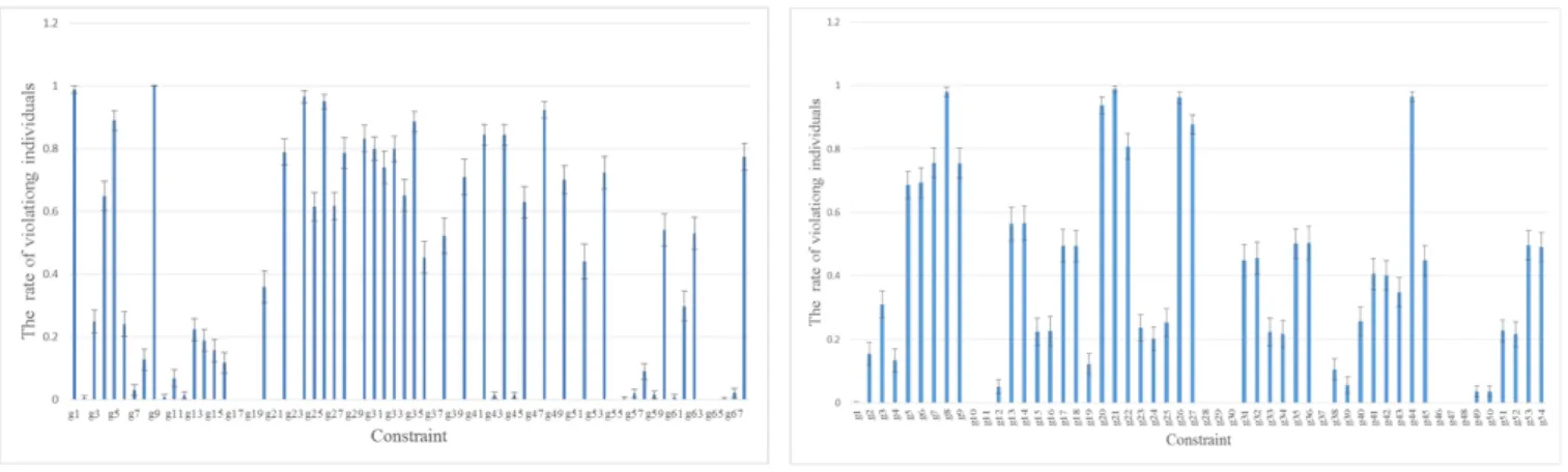
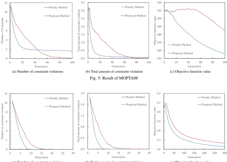
(3) Vol.2018-MPS-119 No.7 2018/7/30. IPSJ SIG Technical Report. Individual 1 Individual 1 Difficult. Easy. Individual 2. Constraint4. Constraint4. Constraint2. Constraint2. Constraint3. Constraint3. Constraint1. Constraint1. vt of individual 2 is smaller than that of 1.. Difficult. Easy. Constraint4. Constraint4. Constraint2. Constraint2. Constraint3. Constraint3. Constraint1. Constraint1. Selected. Selected (a) No individual satisfy the target constraint.. (b) Only one individual satisfies the target constraint.. Individual 1. Individual 1 Difficult. Easy. Individual 2. Individual 2. Difficult. Individual 2. Constraint4. Constraint4. Constraint4. Constraint4. Constraint2. Constraint2. Constraint2. Constraint2. Constraint3. Constraint3. Constraint3. Constraint3. Constraint1. Constraint1. Constraint1. Constraint1. f(x). f(x). Easy. Selected. Selected (c) Some individuals satisfy the target constraint.. (d) Some individuals satisfy all constraints.. Fig. 3: Parent Selection. (a) MOPTA08. (b) Simultaneous design optimization benchmark problem. Fig. 4: Average of violation rate in test problems method were employed in this paper. MOPTA08 has 68 constraints and the simultaneous design optimization benchmark problem has 54 constraints. In MOPTA08, the number of design variables was 124, the population size was 100, the search ended at the 100th generation, the tournament size Ntour was 5 and the penalty factor was 100. The crossover operator was SBX [12] (ηc = 10, Pc = 1.0) and the mutation operator was Polynomial Mutation [12] (ηm = 10, Pm = 1/124). 50 trials were conducted. In the simultaneous design optimization benchmark problem, the number of design variables was 222, the search ended at the 300th generation, the penalty factor was 1 and Pm = 1/222. Other conditions were same with MOPTA08.. ⓒ 2018 Information Processing Society of Japan. 5.2 Difficulty of Constraints In the proposed method, the difficulty of constraints depends on the initial population. It is necessary to confirm how much variation of difficulty of constraints is made for each trial. Fig. 4 shows the average and the standard deviation of violation rate. In both problems, it turns out that the difficulty of constraint were not varied in each trial and were calculated properly. 5.3 Result of MOPTA08 Fig. 5 shows the result of MOPTA08. In the penalty method, as shown in Fig. 5 (a) and (b), there were several constraints which could not be satisfied. The constraints which could not be satisfied were g1 (x) and g9 (x). As shown in Fig. 4, according to the. 3.

(4) Vol.2018-MPS-119 No.7 2018/7/30. IPSJ SIG Technical Report. ϯ͘ϱ. ϭϮ. ϯϮϬ Penalty Method. ϭϬ Number of Constraint. Proposed Method ϴ ϲ ϰ Ϯ Ϭ Ϭ. ϮϬ. ϰϬ ϲϬ Generation. ϴϬ. ϯ͘Ϭ. ϯϭϬ Proposed Method. Objective function value. Total amount of constraint violation. Penalty Method. Ϯ͘ϱ Ϯ͘Ϭ ϭ͘ϱ ϭ͘Ϭ. ϯϬϬ ϮϵϬ ϮϴϬ ϮϳϬ. Ϭ͘ϱ. ϮϲϬ. Ϭ͘Ϭ. ϮϱϬ Ϭ. ϭϬϬ. (a) Number of constraint violations. ϮϬ. ϰϬ ϲϬ Genaration. ϴϬ. ϭϬϬ. Penalty Method Proposed Method Ϭ. (b) Total amount of constraint violation. ϮϬ. ϰϬ ϲϬ Generation. ϴϬ. ϭϬϬ. (c) Objective function value. Fig. 5: Result of MOPTA08. Ϯ͘Ϭ. ϭϮ. ϯ͘Ϯ. Penalty Method. ϭϬ Proposed Method ϴ ϲ ϰ Ϯ. ϭ͘ϲ. Penalty Method ϯ͘ϭ. Proposed Method Objective function value. Total amount of constraint violation. Number of constraint violation. Penalty Method. ϭ͘Ϯ. Ϭ͘ϴ. Ϭ͘ϰ. Ϭ. ϱ. ϭϬ. ϭϱ ϮϬ Generation. Ϯϱ. (a) Number of constraint violations. ϯϬ. ϯ͘Ϭ. Ϯ͘ϵ. Ϯ͘ϴ. Ϯ͘ϳ. Ϭ͘Ϭ. Ϭ. Proposed Method. Ϯ͘ϲ. Ϭ. ϱ. ϭϬ. ϭϱ ϮϬ Generation. Ϯϱ. ϯϬ. (b) Total amount of constraint violation. Ϭ. ϱϬ. ϭϬϬ. ϭϱϬ ϮϬϬ Generation. ϮϱϬ. ϯϬϬ. (c) Objective function value. Fig. 6: Result of simultaneous design optimization benchmark problem difficulty of constraints defined by the proposed method, these two constraints were the most difficult constraints, which were appropriately defined by the initial populations. In the proposed method, the number of constraint violations did not decrease as much as the penalty method in order to satisfy the difficult constraints at the beginning of the search. However, it succeeded in satisfying all constraints including the difficult constraints at the end. As shown in Fig. 5 (c), the objective function was not optimized before all constraints were satisfied because of giving the priority for satisfying constraints. However the objective function was optimized after all constraints were satisfied in the proposed method, which are the features of the proposed method and they worked well. 5.4. Result of simultaneous design optimization benchmark problem Fig. 6 shows the result of the simultaneous design optimization benchmark problem. As shown in Fig. 6 (a) and (b), all methods could satisfy all constraints. However, the proposed method was inferior to the penalty method. It indicates that the proposed method was not effective in the simultaneous design optimization benchmark problem, because there was no local solution in the satisfaction of constraints and considering all constraints simultaneously was more effective in this problem. It can be seen from. ⓒ 2018 Information Processing Society of Japan. Fig. 6 (c), the proposed method was also inferior to the penalty method in the objective function value.. 6.. Conclusion. In this paper, the stepwise satisfaction method of constraints was proposed. This method defines the difficulty of constraints based on the initial population and satisfies the constraints in order of the difficulties. That was realized by giving priority to the individuals satisfying more difficult constraints in the parent selection for crossover. The proposed method and the penalty method were applied to MOPTA08 and the simultaneous design optimization benchmark problem of multiple car structure using response surface method. The results of the experiments showed that the proposed method could satisfy almost all constraints. However, the effectiveness of the proposed method depended on the applied problem. We will analyze the characteristics of the constraints that the proposed method is effective/ineffective and study the combination of the proposed method and the penalty method. Acknowledgments This work was supported by MEXT KAKENHI (Grant-in-Aid for Scientific Research (B), No.16H02889).. 4.

(5) IPSJ SIG Technical Report. Vol.2018-MPS-119 No.7 2018/7/30. References [1] [2] [3]. [4]. [5]. [6]. [7]. [8] [9] [10] [11]. [12]. Dasgupta, D. and Michalewicz, Z.: Evolutionary Algorithms in Engineering Applications, Springer Berlin Heidelberg (2013). Coello, C. and Lamont, G.: Applications of Multi-objective Evolutionary Algorithms, Advances in natural computation, World Scientific (2004). Watanabe, S. and Okudera, M.: A proposal on an approach based on evolutionary multi-criterion optimization for nurse scheduling problem (in Japanese), Transactions of Japanese Society Evolutionary Computation, Vol. 5, No. 3, pp. 32–44 (2014). Mezura-Montes, E. and Coello, C.: Constrained optimization via multiobjective evolutionary algorithms, Multiobjective Problem Solving from Nature, Springer-Verlag Berlin Heidelberg, first edition, pp. 53– 75 (2008). Miyakawa, M. and Sato, H.: Constrained multi-objective optimization using two-stage non-dominated sorting and direct mating (in Japanese), Transactions of Japanese Society Evolutionary Computation, Vol. 5, No. 3, pp. 32–44 (2014). Jain, H. and Deb, K.: An Evolutionary Many-Objective Optimization Algorithm Using Reference-Point Based Nondominated Sorting Approach, Part II: Handling Constraints and Extending to an Adaptive Approach, IEEE Transactions on Evolutionary Computation, Vol. 18, No. 4, pp. 602–622 (2014). Woldesenbet, Y. G., Yen, G. G. and Tessema, B. G.: Constraint Handling in Multiobjective Evolutionary Optimization, IEEE Transactions on Evolutionary Computation, Vol. 13, No. 3, pp. 514–525 (2009). Tanabe, R. and Oyama, A.: A note on constrained multi-objective optimization benchmark problems (in Japanese), Proceedings of Evaluationary Computation Symposium 2016, pp. 340–347 (2016). Homaifar, A., Qi, C. X. and Lai, S. H.: Constrained optimization via genetic algorithms, Simulation, Vol. 62, No. 4, pp. 242–253 (1994). Anjos, M. F.: MOPTA08 benchmark, accessed 2018-1-24, http: //www.miguelanjos.com/jones-benchmark. T. Kohira, H. Kemmotsu, A. O. and Tatsukawa, T.: Proposal of simultaneous design optimization benchmark problem of multiple car structures using response surface method (in Japanese), Transactions of the Japanese Society for Evolutionary Computation, Vol. 8, No. 1, pp. 11–21 (2017). Deb, K. and Goyal, M.: A Combined Genetic Adaptive Search (GeneAS) for Engineering Design, Vol. 26, No. 4, pp. 30–45 (1996).. ⓒ 2018 Information Processing Society of Japan. 5.

(6)