Vol. 62, No. 3, July 2019, pp. 121–131
CORDON AND AREA ROAD PRICING IN RADIAL-ARC NETWORK
Masashi Miyagawa
University of Yamanashi
(Received November 2, 2018; Revised February 6, 2019)
Abstract This paper proposes a continuous network model for determining the size of the toll area and toll level in cordon and area road pricing. Cordon pricing charges a toll to vehicles passing a cordon line surrounding a designated area, whereas area pricing charges a toll to all vehicles driving inside the area. Analytical expressions for the traffic volume and toll revenue are obtained for a circular city with a radial-arc network. The analytical expressions demonstrate how the size of the toll area and toll level affect the traffic volume and toll revenue. Comparing cordon and area pricing shows that area pricing is superior to cordon pricing in both reducing traffic volume in the toll area and generating revenue.
Keywords: Transportation, toll area, toll level, traffic volume, toll revenue, continuous
network model 1. Introduction
Road pricing has attracted attention as a means to reduce traffic congestion. Road pricing encourages travelers to adjust all aspects of their behavior such as number of trips, route, and mode of transport, and thus has a big advantage over other travel demand management policies [4].
The most popular road pricing system is cordon pricing in which vehicles passing a cordon line surrounding a designated area are charged a fixed toll. The cordon pricing has been adopted in Singapore, Stockholm, and Milan. May and Milne [13] compared cordon-based, distance-based, time-based, and delay-based pricing systems. Akiyama et al. [1] compared cordon pricing with congestion pricing on existing toll roads. Sumalee [19] presented a branch-tree framework for finding the optimal cordon location and toll level. A large number of solution methods for the problem have been proposed [5, 18, 25]. Extensions of the problem include multi-layered and multi-centered cordon [26] and time-dependent pricing [7, 27].
Not only cordon pricing but also area pricing has been studied and implemented. In the area pricing, all vehicles driving inside a designated area are charged a fixed toll. Imple-menting the area pricing is thus more difficult than the cordon pricing. The area pricing has been adopted in London. Maruyama and Harata [11] and Maruyama and Sumalee [12] compared the performance of the cordon and area pricing using a trip-chain equilibrium model. Takaki et al. [20] and Takaki et al. [21] developed an algorithm for determining the optimal shape of toll area and toll level. Zheng et al. [28] considered time-dependent area pricing.
Continuous network models have also been used to analyze road pricing. The discrete network models reviewed above aim to develop efficient algorithms applicable to actual road networks, whereas the continuous network models aim to examine fundamental relationships between variables. The continuous models often yield analytical solutions that are easy
to interpret and comprehend, thus supplementing the discrete models. Mun et al. [15] obtained the optimal cordon location and toll level using an urban spatial model of a linear monocentric city. The model was extended by Mun et al. [16] to a non-monocentric city, Verhoef [24] to incorporate land and labor markets, Li et al. [9] to consider the interaction between auto and bus, and Tsai and Lu [22] to multiple-cordon. Ho et al. [6] applied a continuum traffic equilibrium model to the cordon pricing problem in an arbitrary shaped city. Li et al. [10] examined the effect of air pollution cost on the optimal cordon location and toll level in a circular city. In the literature of continuous models, few studies have considered area pricing.
In this paper, we propose a continuous network model for determining the size of the toll area and toll level in cordon and area road pricing. The model yields analytical expressions for the traffic volume and toll revenue, leading to a clear understanding of the basic effect of road pricing. The model will therefore supply building blocks for designing road pricing systems. Other characteristics of the model are as follows. First, the model uses a radial-arc network, which can be found in many cities such as Tokyo, Paris, and Moscow. Second, the model is based on a non-monocentric city where trips occur between any two points in the city. Finally, the model deals with both cordon and area pricing.
The remainder of this paper is organized as follows. The next section develops a radial-arc network model. The following section examines the effects of the size of the toll area and toll level on the traffic volume and toll revenue. The penultimate section compares the cordon and area pricing. The final section presents concluding remarks.
2. Radial-Arc Network Model
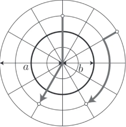
Consider a circular city with radius a, as shown in Figure 1. The city has a dense radial-arc network. A toll area is represented as a circle with radius b located at the center of the city. Cordon pricing charges a toll to vehicles passing or entering the area, whereas area pricing charges a toll to all vehicles driving inside the area. The objectives of road pricing are to reduce the traffic volume in the toll area and to generate the toll revenue. The former directly reduces the traffic congestion in the area, whereas the latter indirectly reduces the traffic congestion by using the revenue to improve infrastructure.
Let t be the toll level and α be the travel cost per unit distance. The travel cost C for trips of length R is defined as
C = αR + t. (2.1)
Every traveler is assumed to use the least cost route. Since the travel cost also depends on the travel time in practice, this assumption can be applied to the case where the travel speed is regarded as constant throughout the city. If no toll is charged, i.e., t = 0, the travel distance R is reduced to the radial-arc distance. The radial-arc distance S between two points (r1, θ1) and (r2, θ2) in the polar coordinate is defined as
S =
{
|r1− r2| + min{r1, r2}φ, 0 ≤ φ < 2,
r1+ r2, 2≤ φ ≤ π,
(2.2) where φ = min{|θ1 − θ2|, 2π − |θ1 − θ2|} [8]. Both radial and arc roads are used if φ < 2, whereas only radial roads are used if φ≥ 2, as shown in Figure 1. The radial-arc distance is a good approximation for the actual travel distance in cities with a radial-arc network [23]. The travel demand D depends on the travel cost and is expressed as
where D0 is the travel demand when C = 0 and β (> 0) is a parameter for elasticity. The travel demand decreases with the trip length R and the toll level t. The exponential function, which is common in spatial interaction models [17], allows us to obtain analytical expressions for the traffic volume and toll revenue.
Assume that origins and destinations are uniformly distributed in the city. The uniform distribution serves as a basis for further analysis with more realistic distributions. In fact, the uniform distribution has frequently been used in continuous transportation models [2, 3, 14]. The traffic in the city is classified into four groups according to the location of origin and destination. If both origin and destination are outside the toll area, the traffic is called
through traffic. If origin is outside (inside) the toll area and destination is inside (outside)
the toll area, it is called inward (outward ) traffic. If both origin and destination are inside the toll area, it is called city traffic.
a
b
Figure 1: Circular city with a radial-arc network
3. Traffic Volume and Toll Revenue
In this section, we examine the effects of the size of the toll area and toll level on the volume of through, inward, outward, and city traffic, and the toll revenue by each traffic.
Let (r1, θ1) (b ≤ r1 ≤ a, 0 ≤ θ1 < 2π) and (r2, θ2) (b ≤ r2 ≤ a, 0 ≤ θ2 < 2π) be origin and destination of through traffic, respectively. Through traffic passes the toll area if the travel cost of passing the toll area is smaller than that of making a detour around the toll area. The condition of passing the toll area is then
2αb + t ≤ αbφ ⇔ φ ≥ t
αb + 2. (3.1)
Travel routes for trips of θ1 = 0 are shown in Figure 2a. Through traffic passes the toll area if destination is inside the gray region in the figure. The travel cost of through traffic passing the toll area CT is given by
CT = α(r1+ r2) + t. (3.2) Substituting into (2.3) and integrating with respect to r1, θ1, r2, and θ2 yield the volume of through traffic passing the toll area
VT = ∫ 2π 0 ∫ a b ∫ π t/(αb)+2 ∫ a b 2D0exp[−β{α(r1+ r2) + t}]r1r2dr2dθ2dr1dθ1 = 4πD0 α4β4 ( π− 2 − t αb )
{(αβb + 1)eαβa− (αβa + 1)eαβb}2
The volume of through traffic passing the toll area VT is shown in Figure 2b, where a = 1, D0 = 1, α = 1, β = 1. If the toll area is small, much traffic passes the toll area at t = 0 but VT decreases rapidly with t. On the other hand, if the toll area is large, VT is small at
t = 0 but decreases gradually with t, and thus a higher toll is required to reduce the volume
of through traffic passing the toll area. The toll level that achieves VT = 0 is
t†= (π− 2)αb, (3.4)
which is proportional to the radius of the toll area b. The toll revenue by through traffic
TT = tVT is shown in Figure 2c. The toll revenue has a maximum between t = 0 and t = t†. The toll level that maximizes the toll revenue by through traffic is
tT = (π− 2)αβb + 2 − √
(π− 2)2α2β2b2+ 4
2β . (3.5)
As the toll area becomes larger, a higher toll is required to maximize the toll revenue. Since both t† and tT depend on b, the size of the toll area and toll level should be determined simultaneously. 0 0.2 0.4 0.5 0.6 1.5 0.8 1.0 2.0 1.0 t b=0.2 b=0.4 b=0.6 VT t αb 0 0.1 0.2 0.5 0.3 1.5 0.4 1.0 2.0 0.5 t T b=0.2 b=0.4 b=0.6 T (a) (c) (b) 2
Figure 2: (a) Routes of through traffic; (b) Volume of through traffic passing the toll area; (c) Toll revenue by through traffic
As shown in Figure 2a, if 2 < φ < t/(αb) + 2, through traffic makes a detour around the toll area. The travel cost of through traffic making a detour CU is given by
Substituting into (2.3) and integrating with respect to r1, θ1, r2, and θ2 yield the volume of through traffic making a detour
VU = ∫ 2π 0 ∫ a b ∫ t/(αb)+2 2 ∫ a b 2D0exp[−αβ{r1+ r2+ b(θ2− 2)}]r1r2dr2dθ2dr1dθ1 = 4πD0 α5β5b(e
βt− 1){(αβb + 1)eαβa− (αβa + 1)eαβb}2e−β{2α(a+b)+t}. (3.7)
The volume of through traffic making a detour VU is shown in Figure 3. It can be seen that VU increases with t and then becomes constant. This means that if t > t†, all through traffic makes a detour around the toll area. Since this detour traffic passes the boundary of the toll area, the increase in the traffic volume should be considered when designing road pricing. 0 0.2 0.4 0.5 0.6 1.5 0.8 1.0 2.0 1.0 t b=0.2 b=0.4 b=0.6 VU
Figure 3: Volume of through traffic making a detour
Let (r1, θ1) (b ≤ r1 ≤ a, 0 ≤ θ1 < 2π) and (r2, θ2) (0 ≤ r2 ≤ b, 0 ≤ θ2 < 2π) be origin and destination of inward traffic, respectively. Travel routes for trips of θ1 = 0 are shown in Figure 4a. The travel cost of inward traffic CI is given by
CI= {
α(r1− r2+ r2θ2) + t, 0≤ θ2 < 2,
α(r1+ r2) + t, 2≤ θ2 ≤ π.
(3.8) Substituting into (2.3) and integrating with respect to r1, θ1, r2, and θ2 yield the volume of inward traffic VI= ∫ 2π 0 ∫ a b ∫ 2 0 ∫ b 0 2D0exp[−β{α(r1− r2+ r2θ2) + t}]r1r2dr2dθ2dr1dθ1 + ∫ 2π 0 ∫ a b ∫ π 2 ∫ b 0 2D0exp[−β{α(r1+ r2) + t}]r1r2dr2dθ2dr1dθ1 = 4πD0 α4β4 {(π − 3 + e αβb )(eαβb− 1) − (π − 2)αβb}
{(αβb + 1)eαβa− (αβa + 1)eαβb}e−β{α(a+2b)+t}. (3.9)
The volume of inward traffic VI and the toll revenue by inward traffic TI= tVI are shown in Figures 4b and 4c, respectively. As the toll area becomes larger, both VIand TIincrease. The toll level that maximizes the toll revenue by inward traffic is
tI= 1
(a) (c) (b) 2 0 0.2 0.4 0.5 0.6 1.5 0.8 1.0 2.0 1.0 t VI b=0.2 b=0.4 b=0.6 0 0.1 0.2 0.5 0.3 1.5 0.4 1.0 2.0 0.5 t T b=0.2 b=0.4 b=0.6 I
Figure 4: (a) Routes of inward traffic; (b) Volume of inward traffic; (c) Toll revenue by inward traffic
which is independent of the size of the toll area.
The volume of outward traffic VO is the same as that of inward traffic, i.e.,
VO = VI. (3.11)
Let (r1, θ1) (0 ≤ r1 ≤ b, 0 ≤ θ1 < 2π) and (r2, θ2) (0 ≤ r2 ≤ b, 0 ≤ θ2 < 2π) be origin and destination of city traffic, respectively. Travel routes for trips of θ1 = 0 are shown in Figure 5a. The travel cost of city traffic CC is given by
CC = α(r1− r2+ r2θ2) + t, r1 ≥ r2, 0≤ θ2 < 2, α(r2− r1+ r1θ2) + t, r1 < r2, 0≤ θ2 < 2, α(r1+ r2) + t, 2≤ θ2 ≤ π. (3.12)
city traffic VC = ∫ 2π 0 ∫ b 0 ∫ 2 0 ∫ r1 0 2D0exp[−β{α(r1 − r2+ r2θ2) + t}]r1r2dr2dθ2dr1dθ1 + ∫ 2π 0 ∫ b 0 ∫ 2 0 ∫ b r1 2D0exp[−β{α(r2− r1+ r1θ2) + t}]r1r2dr2dθ2dr1dθ1 + ∫ 2π 0 ∫ b 0 ∫ π 2 ∫ b 0 2D0exp[−β{α(r1+ r2) + t}]r1r2dr2dθ2dr1dθ1 = 2πD0 α4β4 [2α 2β2b2(π− 2 + e2αβb) + (eαβb− 1){5 − 2π + (2π − 11)eαβb} − 2αβb{5 − 2π + 2(π − 4)eαβb}]e−β(2αb+t). (3.13)
The volume of city traffic VC and the toll revenue by city traffic TC = tVC are shown in Figures 5b and 5c, respectively. If the toll area is small, the toll level has little impact on
VC and TC because VC is small even at t = 0. As the toll area becomes larger, both VC and TC increase. The toll level that maximizes the toll revenue by city traffic is
tC = 1 β. (3.14) (a) (c) (b) 2 0 0.2 0.4 0.5 0.6 1.5 0.8 1.0 2.0 1.0 t VC b=0.2 b=0.4 b=0.6 0 0.1 0.2 0.5 0.3 1.5 0.4 1.0 2.0 0.5 t T b=0.2 b=0.4 b=0.6 C
4. Cordon and Area Pricing
Cordon pricing charges a toll to through and inward traffic, whereas area pricing charges a toll to all traffic including outward and city traffic. In this section, we compare the cordon and area pricing in terms of the traffic volume in the toll area and toll revenue.
The traffic volume for cordon pricing is given by the sum of VT, VI, VO, and VC, where
t = 0 for VO and VC. The traffic volume and toll revenue are shown in Figures 6a and 6b, respectively. Note that both curves have kinks at t = t† where the volume of through traffic becomes zero. Note also that the toll revenue has a maximum at t∗ = 1/β = 1. These figures provide planners with alternatives for the size of the toll area and toll level. To completely eliminate through traffic from the toll area, the toll level should be set at t = t†. To reduce the total traffic volume in the toll area, a higher toll may be required because the traffic volume decreases gradually with t. If generating revenue is the most important, the toll area should be large and the toll level should be set at t = t∗.
(b) (a) 0 1.0 1.5 0.5 0.5 2.0 1.5 2.5 1.0 2.0 3.0 t V b=0.2 b=0.4 b=0.6 0 0.2 0.4 0.5 0.6 1.5 0.8 1.0 2.0 1.0 t T b=0.2 b=0.4 b=0.6
Figure 6: (a) Traffic volume for cordon pricing; (b) Toll revenue for cordon pricing The traffic volume for area pricing is given by the sum of VT, VI, VO, and VC. The traffic volume and toll revenue for area pricing are shown in Figures 7a and 7b, respectively. Note that as the toll level increases, the traffic volume for area pricing decreases more rapidly than that for cordon pricing. Note also that the toll revenue for area pricing, which has a maximum at t∗ = 1/β = 1, is greater than that for cordon pricing. It follows that area pricing is superior to cordon pricing in both reducing traffic volume in the toll area and generating revenue. This is consistent with the result of case studies using actual road networks and traffic data [11, 12].
5. Conclusions
This paper has presented a continuous network model for determining the size of the toll area and toll level in road pricing. The traffic volume and toll revenue have been obtained for a circular city with a radial-arc network. Cordon and area pricing have then been compared in terms of the traffic volume in the toll area and toll revenue.
The model is useful for road pricing design as follows. First, the analytical expressions for the traffic volume and toll revenue demonstrate the effects of the size of the toll area and toll level. Note that finding these relationships by using discrete network models requires computation of the traffic volume for various combinations of the parameters. These rela-tionships help planners to estimate the size of the toll area and toll level required to achieve a certain level of traffic volume and toll revenue. Second, the model explicitly considers
(b) (a) 0 1.0 1.5 0.5 0.5 2.0 1.5 2.5 1.0 2.0 3.0 t V b=0.2 b=0.4 b=0.6 0 0.2 0.4 0.5 0.6 1.5 0.8 1.0 2.0 1.0 t T b=0.2 b=0.4 b=0.6
Figure 7: (a) Traffic volume for area pricing; (b) Toll revenue for area pricing
through, inward, outward, and city traffic, thereby allowing us to examine how the traffic composition affects the traffic volume and toll revenue. Finally, comparing cordon and area pricing shows that area pricing is superior to cordon pricing in both reducing traffic volume in the toll area and generating revenue. This result provides a fundamental understanding of road pricing and gives an insight into discrete network models for empirical analysis.
To obtain analytical expressions, the present model has many simplifying assumptions. Future research should extend the model to incorporate non-uniform distribution of origins and destinations, travel demand based on trip-chain, and multi-layered cordon.
Acknowledgements
This research was supported by JSPS KAKENHI Grant Numbers JP18K04604, JP18K04628. I am grateful to anonymous reviewers and the editor for their helpful comments and sug-gestions.
References
[1] T. Akiyama, S. Mun, and M. Okushima: Second-best congestion pricing in urban space: Cordon pricing and its alternatives. Review of Network Economics, 3 (2004), 401–414.
[2] S. Chien and P. Schonfeld: Optimization of grid transit system in heterogeneous urban environment. Journal of Transportation Engineering, 123 (1997), 28–35.
[3] C.F. Daganzo: Structure of competitive transit networks. Transportation Research
Part B, 44 (2010), 434–446.
[4] A. de Palma and B. Lindsey: Traffic congestion pricing methodologies and technologies.
Transportation Research Part C, 19 (2011), 1377–1399.
[5] J. Ekstr¨om, A. Sumalee, and H.K. Lo: Optimizing toll locations and levels using a mixed integer linear approximation approach. Transportation Research Part B, 46 (2012), 834–854.
[6] H.W. Ho, S.C. Wong, H. Yang, and B.P.Y. Loo: Cordon-based congestion pricing in a continuum traffic equilibrium system. Transportation Research Part A, 39 (2005), 813–834.
[7] I. Kristoffersson: Impacts of time-varying cordon pricing: Validation and application of mesoscopic model for Stockholm. Transport Policy, 28 (2013), 51–60.
[8] O. Kurita: Theory of road patterns for a circular disk city: Distributions of Euclidean, recti-linear, circular-radial distances. Journal of the City Planning Institute of Japan,
36 (2001), 859–864 (in Japanese).
[9] Z.-C. Li, W.H.K. Lam, and S.C. Wong: Modeling intermodal equilibrium for bimodal transportation system design problems in a linear monocentric city. Transportation
Research Part B, 46 (2012), 30–49.
[10] Z.-C. Li, Y.-D. Wang, W.H.K. Lam, A. Sumalee, and K. Choi: Design of sustainable cordon toll pricing schemes in a monocentric city. Networks and Spatial Economics, 14 (2014), 133–158.
[11] T. Maruyama and N. Harata: Difference between area-based and cordon-based conges-tion pricing: Investigaconges-tion by trip-chain-based network equilibrium model with nonad-ditive path costs. Transportation Research Record, 1964 (2006), 1–8.
[12] T. Maruyama and A. Sumalee: Efficiency and equity comparison of cordon- and area-based road pricing schemes using a trip-chain equilibrium model. Transportation
Re-search Part A, 41 (2007), 655–671.
[13] A.D. May and D.S. Milne: Effects of alternative road pricing systems on network performance. Transportation Research Part A, 34 (2000), 407–436.
[14] M. Miyagawa: Optimal allocation of area in hierarchical road networks. The Annals
of Regional Science, 53 (2014), 617–630.
[15] S. Mun, K. Konishi, and K. Yoshikawa: Optimal cordon pricing. Journal of Urban
Economics, 54 (2003), 21–38.
[16] S. Mun, K. Konishi, and K. Yoshikawa: Optimal cordon pricing in a non-monocentric city. Transportation Research Part A, 39 (2005), 723–736.
[17] J.R. Roy: Spatial Interaction Modelling (Springer-Verlag, Berlin, 2010).
[18] S. Shepherd and A. Sumalee: A genetic algorithm based approach to optimal toll level and location problems. Networks and Spatial Economics, 4 (2004), 161–179.
[19] A. Sumalee: Optimal road user charging cordon design: A heuristic optimization approach. Computer-Aided Civil and Infrastructure Engineering, 19 (2004), 377–392. [20] R. Takaki, T. Maruyama, and S. Mizokami: The optimal area-based network congestion
pricing problem: Development and applications of algorithm for determining optimal toll level and charging boundary. Journal of Japan Society of Civil Engineers, 67 (2011), 1233–1242 (in Japanese).
[21] R. Takaki, T. Maruyama, and S. Mizokami: Optimal network congestion pricing design problem controlling the shape of charging boundary: Algorithm development and appli-cations. Journal of Japan Society of Civil Engineers, 70 (2014), 88–101 (in Japanese). [22] J.-F. Tsai and S.-Y. Lu: Reducing traffic externalities by multiple-cordon pricing.
Transportation, 45 (2018), 597–622.
[23] R.J. Vaughan: Urban Spatial Traffic Patterns (Pion, London, 1987).
[24] E.T. Verhoef: Second-best congestion pricing schemes in the monocentric city. Journal
of Urban Economics, 58 (2005), 367–388.
[25] L. Zhang and J. Sun: Dual-based heuristic for optimal cordon pricing design. Journal
of Transportation Engineering, 139 (2013), 1105–1116.
[26] X. Zhang and H. Yang: The optimal cordon-based network congestion pricing problem.
[27] N. Zheng, R.A. Waraich K.W. Axhausen, and N. Geroliminis: A dynamic cordon pricing scheme combining the macroscopic fundamental diagram and an agent-based traffic model. Transportation Research Part A, 46 (2012), 1291–1303.
[28] N. Zheng, G.R´erat, and N. Geroliminis: Time-dependent area-based pricing for multi-modal systems with heterogeneous users in an agent-based environment. Transportation
Research Part C, 62 (2016) 133–148.
Masashi Miyagawa
Department of Regional Social Management University of Yamanashi
4-4-37 Takeda, Kofu
Yamanashi 400-8510, Japan