東北大学機関リポジトリTOUR

Behavioristic Perspective

著者

WANG RENHAO

学位授与機関

Tohoku University

学位授与番号

11301甲第18251号

Essays on Market Anomalies from a

Behavioristic Perspective

A Dissertation Presented to

Graduate School of Economics and Management, Tohoku University

in particular

fulfillment of the requirements for the

degree of Doctor of Philosophy

by Wang Renhao

ACKNOWLEDGEMENT

I would like to express my most genuine gratitude to everyone who has offered great contributions to this work.

Firstly, and most sincerely, I thank Professor Jiro Akita wholeheartedly. It will be impossible for me to finish this dissertation without his patient and kindness help. Studying under Professor Akita’s guidance, my Ph.D. has been an amazing experience, not only for his tremendous academic support but also for the critical thinking I learned and benefited from him.

Similar, profound gratitude goes to the members of my dissertation committee: Professor Akiomi Kitagawa and Professor Hiroaki Chigira. They have generously offered their time, support, guidance, and goodwill throughout the preparation and review of this document. I also wish to thank my best friend, Doctor Mi Xianhua, for his great assistance with the mathematics deduction which is essential to this study.

Finally, thanks go to my family and my friends for almost unbelievable support. Especially, for my uncle and aunt who inspired and encouraged me to pursue a high academic accomplishment; for my brother and my sister in law who take the responsibility of looking after the family, which I failed to; for my grandparents and parents who raised me as a man with will. They are the most important people in my world, and I dedicate this thesis to them.

ABSTRACT

In this thesis, we try to understand the volatility anomaly and the trading volume anomaly in the financial market by one of the most important behavioristic biases investors are facing, their extrapolation belief.

Firstly, we use the empirical test to investigate if investor’s extrapolation belief can significantly impact the volatility and trading volume. According to the recent groundbreaking work of Greenwood and Shleifer (2014), extrapolation investors’ expected return is “a weighted average of past returns.” Therefore, we construct the Greenwood Shleifer Index(GSI) to quantitatively represent investors’ extrapolative belief. Then we use this index as an explaining variable to test its relation to the volatility and trading volume of different financial markets.

Chapter 1 represents our empirical test results about the relation between GSI and

volatility. It is shown in this chapter that in most of the financial markets, GSI can significantly impact volatility even if we include economic factors in our regression, indicating the changing extrapolation belief could be a reason causing volatility to change, especially when individual investors dominate the market. We also find an asymmetric GSI-volatility relationship that volatility is more easily affected by individuals’ extrapolation belief during the declining market.

In the light of previous extrapolative models, Chapter 2 builds a new model to explain the empirical finding of Chapter 1. In our new model, extrapolative investors also pay attention to information innovations, but with confirmation bias when they

evaluate the new arriving information. By questionnaire survey, we give direct evidence that confirmation bias and extrapolation bias could impact individual investors simultaneously. Then by analytical proportions and numerical simulation, we show our model can provide specific links between volatility and investors’ extrapolation belief. Additionally, we find our theory can also help us to explain one of the most stylized facts of volatility, the volatility clustering.

Chapter 3 seeks the relation between GSI and trading volume. Using simple ARIMA

structure regression tests, we find individuals’ extrapolation belief can significantly impact the trading volume, but the effect is different according to different market. Specifically, in the emerging stock market where short-sale constraint exists, when GSI<0, trading volume is negatively correlated with |GSI|, the magnitude of individuals’ extrapolation belief, but when GSI>0, trading volume is positively correlated with |GSI|. On the contrary, trading volume is positively correlated with |GSI| for both positive and negative GSI in the future market, where investors are free to sell short. The reason for this wacky relationship is in need of further discussion.

Chapter 4 tries to explain this confusing relation between trading volume and

individuals’ extrapolation belief. We find that with a simple modification, our model in

Chapter 2 can efficiently explain this intriguing relation. The only modification we

make is that extrapolators are heterogeneous with each other in the way that every extrapolator has his idiosyncratic bias when evaluating the information innovations. In this new model, their heterogeneity is amplified by their extrapolation belief. We prove

magnitude of individuals’ extrapolation belief grows. On the contrary, during the bear market, in the emerging stock market, extrapolators gradually quit the market as |#$%| increases, the market is left will only fundamentalists who are homogenous with each other, the trading volume reduces accordingly. Moreover, using simulation, we show that our model can effetely explain the most two important features of financial bubbles: the high trading volume, and the high volatility. Volatility rises because extrapolator’s expectation is becoming more volatile, trading volume increases as extrapolators are getting more heterogeneous with their peers.

To summarize, this thesis makes several contributions. Firstly, this thesis is the first one to empirically investigate the relationship between volatility, trading volume and individuals’ extrapolation bias. Secondly, we confirmed some stylized facts that previous researches are missing, the asymmetric GSI-volatility relationship, for example. Thirdly, we build a new extrapolative model which not only can help us to understand the trading volume and volatility in financial markets but also gives a better explanation for the financial bubbles. We also suggest it may be a more promising way to study irrational individual investors’ behavior from multiple angles, like what we did in building the new model.

TABLE OF CONTENTS ACKNOWLEDGEMENT ... i ABSTRACT ... ii LIST OF TABLES ... viii LIST OF FIGURES ... x 1. The time-varying Volatility and Extrapolation Belief ... 1 1.1 Introduction ... 1 1.2 Literature Review ... 8 1.3 Data and Descriptive Statistics ... 10 1.4 Calculation Method and Result Discussion ... 13 1.4.1 Index calculation method ... 13 1.4.3 Empirical Test Result and Comparison of different markets ... 19 1.4.3 Result comparison of different stages ... 23 1.5 Further Discussion ... 26 Appendix 1 ... 36 2. Extrapolation, Confirmation Bias and Volatility ... 49 2.1 Introduction ... 49 2.2 Questionnaire Survey ... 57 2.3 The model ... 63

2.3.2 Equilibrium Price and implications ... 71 2.3.3 Volatility Clustering ... 76 2.3.4 Asymmetric Relation between Extrapolation Belief and Volatility ... 78 2.4 High-frequency simulation ... 79 2.4.1 Simulation mothed ... 80 2.4.2 Numerical Simulation result ... 83 2.5 Conclusion ... 88 Appendix 2.1 ... 93 Appendix 2.2 ... 94 Appendix 2.3 Questionnaire ... 104 3. Extrapolation Belief and the Trading Volume ... 106 3.1 Introduction ... 106 3.2 Literature Review ... 111 3.3 Empirical test ... 114 3.2.1 Data description and Empirical methodology ... 114 3.2.2 Empirical test result ... 118 3.4 Conclusion and Discussion ... 121 Appendix 3 ... 127 4. Extrapolation Belief, Trading Volume and Bubbles ... 137 4.1 Introduction ... 137 4.2 Literature Review ... 142

4.3 A New Model with Heterogeneous Extrapolators ... 145 4.3.1 No short-sale constraint ... 148 4.3.2 Short-sale constraint ... 151 4.4 Simulation of the bubble ... 165 4.4.1 Simulation of the basic model ... 166 4.4.2 Simulated Acceptable Price of different investors ... 170 4.6 Conclusion ... 171 Appendix 4.1 ... 177 Appendix 4.2 ... 182

LIST OF TABLES

Table 2.5 Investors’ behavior survey statistics ... 101 Table 2.6 Summary of empirical results in different financial market ... 102 Table 2.7 Comparison of Correlations between |GSI| and Volatility ... 103 Table 3.1 Stationary test for logarithm value of trading volume (log (Volumet)) ... 128 Table 3.2 Empirical results for IXIC with ARIMA (1,0,1) structure for different λ ... 129 Table 3.3 Empirical results for GEI with ARIMA (1,1,1) structure for different λ ... 130 Table 3.4 Empirical results for SSEC with ARIMA (3,1,1) structure for different λ ... 131 Table 3.5 Empirical results for Shanghai Silver Future with ARIMA (1,1,1) structure for different λ ... 132 Table 3.6 Empirical results for Shanghai Gold Future with ARIMA (1,1,1) structure for different λ ... 133 Table 3.7 Empirical results for Brent Crude Oil Future with ARIMA (1,0,2) structure for different λ ... 134 Table 3.8 Summary of empirical results in different financial market ... 135 Table 4.2: Numerical benchmark parameters for bubble simulation ... 166 Table 4.1: Selected models of bubbles ... 177

LIST OF FIGURES

Figure 2.8 Correlation and Changing proportion of extrapolators ... 96 Figure 2.9 volatility clustering in real financial markets and by our simulation result .... 97 Figure 3.1 Stock traded, turnover ratio of domestic shares ... 127 Figure 3.2 Changing Hands of Shanghai Stock Market ... 127 Figure 3.3 Changing Hands of Chinese Gold Future Market ... 128 Figure 4.1 Demonstration of price evolution in the bull market ... 156 Figure 4.2 Demonstration of price evolution in the bear market ... 162 Figure 4.3 Simulation result of a financial bubble ... 179 Figure 4.4 The changing demand of investors ... 179 Figure 4.5 Evolution of extrapolators’ Acceptable Price ... 180 Figure 4.6 Histogram of extrapolators’ Acceptable Price ... 181

1. The time-varying Volatility and Extrapolation Belief

Abstract: This paper empirically studies the relationship between the time-varying volatility and individual’s extrapolation belief in several financial markets. Based on the groundbreaking work of Greenwood and Shleifer (2014) that extrapolative investors’ expected return is a weighted average of previous returns, we construct the Greenwood Shleifer Index(GSI) to represent investors’ extrapolative belief. Results of our empirical test indicate the changing extrapolation belief could be a reason causing volatility to change, especially when individual investors dominate the market. We also find an asymmetric GSI-volatility relationship that volatility is more easily affected by individuals’ extrapolation belief during the declining market.

1.1 Introduction

Volatility, which is thought to be one of the most essential benchmarks of the financial market, changes over time (Fama (1965), Castanias (1979)). There are a lot of scholars attempting to understand the fluctuation in volatility from the view of economic factors. For example, Flannery and Protopapadakis (2002) try to investigate the relation between the conditional volatility and macroeconomic variables, but just find valid results for only a small part of economic variables they are using. Other researchers, including Cutler, Poterba, and Summers (1990), Fleming and Remolona

(1999), Andersen and Bollerslev (1998), Andersen et al. (2003), try to relate volatility changes in the stock market to micro-economic factors that can affect expected returns. Recent works like Engle and Rangel (2008), Christiansen et al. (2012), Mittnik, Spindler and Robinzonov (2015) try to use more sophisticated models like Spine-Garch to revisit how can stock market volatility be affected by macroeconomic activities. But they only find similar conclusions that the economic factors have limited power in explaining the movements in stock volatility (Mittnik, Spindler, and Robinzonov (2015)).

Instead of paying attention to economic factors, this paper tries to seek the relationship between the time-varying volatility and one of the most important individual investors’ biases, their extrapolation belief. By empirical tests, this paper shows that volatility index is highly correlated with the extent of investors’ extrapolation belief in most financial markets. We believe individual investors’ extrapolation behavior can help us to understand the fluctuation in volatility from a new perspective.

Extrapolation means investors tend to form their expectation of future returns by previous price trend (Barberis et al. (2016)). They believe the stock price will always keep its trend—the price will continue to rise if it has a positive cumulative price change, and vice versa. Both psychology papers and financial literature provide evidence proving that extrapolation bias can deeply impact people’s decision-making process (see, Gilovich et al. (1985); Hirshleifer (2001); Barberis and Thaler, (2003); Fuster et

for many capital market phenomenon, e.g., the overreaction anomalies (Barberis et al., (1998)), the bubble generation (Barberis et al., (2016)), herding investment (Barberis and Shleifer (2003)) and so on.

Recently, a groundbreaking development of extrapolation theory is given by Greenwood and Shleifer (2014). They use survey evidence from multiple resources, empirically prove that “investors’ extrapolative belief is a weighted average of past price changes, where more recent price changes are weighted more heavily.” Based on their work, this paper structures Greenwood and Shleifer Index (GSI) to quantitatively measure the extent of extrapolation belief of investors. We choose daily market data from several kinds of financial markets, including emerging stock markets (Chinese stock market), developed stock markets, the Brent crude oil future market, and the currency markets (JPYUSD and EURUSD), to empirical seek its impact on movements in volatility.

To characterize the time varying volatility, this paper applies the Realized Volatility method using 5-min high frequency intraday data. Then we use a simple least squares regression model to investigate if volatility is related to individuals’ extrapolation belief. This paper also distinguishes positive GSI from negative GSI with two dummy variables to explore the possible asymmetric influence in raising market and in declining market. Besides, to eliminate possible spurious regression, we also introduce economic factors into our equitation, to see if the regression result will change significantly.

Strikingly, we find significant regression result that GSI, no matter positive or negative, and no matter with or not without economic factors, does statistically affect volatility index for most of the financial markets. Besides, all the regression results are much better when we include GSI as explaining variables than those with only economic factors. These regression results strongly prove that extrapolation is a reason causing volatility to change.

Besides, it can also be seen from our test that when individual investors take a bigger fraction of the whole population, the relationship between GSI and volatility get closer. For example, the Chinese stock market, with its reputation for “individual investors dominated immature market”, has the biggest individual trading volume proportion as well as the best regression result. On the contrary, no significant correlation between GSI and volatility index can be found in the currency market where individual investors only trade a very small proportion of the whole amount. When individual investors’ proportion maintains a moderate size, like Japanese stock market, Nasdaq stock market and the Brent Crude future market, only weak significant regression result can be discovered. Besides, the significance of the estimated parameter of both positive GSI and negative GSI holds even if we include macroeconomic factors in our empirical test. These empirical results indicate that volatility is indeed influenced by individuals’ extrapolation belief.

These diverse empirical test results of different markets can be explained from the different characters of market participators. Individual investors, also called as “retail

and make detrimental investment decisions (Barber and Odean (2011), De long et. al. (1990), Shefrin and Thaler (2004), Shiller (2015)). Extrapolation, of course, is one of the most pervasive ones. De Bondt (1998), for example, argues that “Perhaps the best-established stylized fact is extrapolation bias...” Institutional investors, on the contrary, are supposed to have the ability to get all information and correctly evaluate the fundamental price of equity which can help them to arbitrage the mispricing away (Fama (1965), Black (1972), Huberman (2005)). But recent empirical and theoretical findings show that, when the market is filled with enthusiastic extrapolators, institutional investors may not trade against them, or, in some circumstances, they will even try to ride the bubble, buy in asset which they believe it is already over-priced and hoping to sell it to latter arriving irrational investors who will buy the asset in an even higher price (De Long et al. 1990, Abreu and Brunnermeier 2003, Brunnermeier and Nagel 2004). So, a higher proportion of individual trading will indicate a bigger influence of extrapolation belief to the price, therefore a better explanatory power of GSI to volatility index.

To test the robustness of the effect that individual investors’ proportion has on the explanatory power of GSI to volatility index, this paper goes further to compare the regression results between the two indexes in different stages of the same market by dividing the samples of Chinese stock market into core-bubble stage and non-core stage. During bubbles, the extraordinary enthusiasm of individual investors keeps them rushing into the market and becoming more active (Shiller 2015), individual investors will take a bigger proportion as well as a higher influence to the market. Hence,

individual investors’ irrational behavior will have a more notable impact on the market, and volatility should also have a closer relation with GSI. As a result, our test confirms this conjecture. For all three samples of Chinese stock market, we do find better regression result in core-bubble stages than in non-bubble stages — after casting the bubble period, the rest of the sample only show poor fitting effect while the core-bubble stage samples still have highly significant regression results.

According to these comparisons, we may cautiously get the conclusion that changes in extrapolation belief can be one of the reasons causing volatility to change, especially when individual investors take a big proportion of the market.

Besides, our test gives clear evidence of the asymmetric relationship between GSI and volatility. To begin with, our empirical result shows the regression coefficients of the negative GSI are bigger than the coefficient of the positive GSI for all the samples. Also, the coefficient significance level of negative GSI is much higher. When GSI>0, the regression coefficient is only highly significant in Chinese stock market, which turns to weakly significant for other markets. Especially for Nasdaq stock market, where we cannot find significant relation between positive GSI and volatility. Contrarily, coefficient of negative GSI is still highly significant (p<0.01) across all the samples (except currency market). These results demonstrate the asymmetric GSI-volatility relation that GSI-volatility is more easily affected by individuals’ extrapolation belief during declining market, but during bull market, this relation is weaker.

across time from the perspective of individuals’ extrapolation bias. Although many behavioral papers have documented how individuals’ irrational behaves can exaggerate volatility (DeLong et. al. (1990), Odean (1998), Scheinkman and Xiong (2003), Barberis, Greenwood and Shleifer (2015)), most of these works are focusing on why volatility is “excess” relative to predictions of standard theory model, i.e. the “excess volatility puzzle” of Shiller (Shiller 1980, LeRoy and Porter 1981). Few of them try to study the time-varying nature of volatility from behavioral perspective (for more detail, see Section 1.2). This paper shows that individuals’ irrational bias can not only account for “excess volatility”, but can also drive volatility to change across time.

Secondly, our finding is an important supplement to researches about the changing volatility. As demonstrated above, previous papers mainly try to explain the fluctuation in volatility with economic factors. Pitifully, according to their results, the economic factors can only explain small part of the movements in volatility (Bollerslev, Engle, and Wooldridge (1988), Schwert (1989), Christiansen et. al. (2012), Mittnik, Spindler and Robinzonov (2015)). But according to this paper’s result, volatility index is correlated with extrapolation belief in most of the markets, even for the well-developed stock markets such as Nasdaq stock market and Japanese stock market. Therefore, people’s irrational bias (extrapolation belief in our paper) can be other factors causing volatility to change. That is what previous paper doesn’t take into account. Thus, it is more suitable to understand the volatility fluctuation by combining economic factors and people’s irrational behave.

However, we cannot find satisfying theoretical explanations for this empirical result in previous papers. It is the only thing emphasized in previous papers that Extrapolation, as a bias, can affect individual’s expectation about future returns, which also becomes the starting point for previous papers to explain market anomalies such as the generation of financial bubbles, overreaction (Barberis et al. (2016), Hong and Stein (1999)). But, most of these papers describe extrapolation of investors is a deterministic process—it is only determined by past returns. Therefore, there is no fluctuation in individuals’ extrapolation belief in these models. Nevertheless, according to our empirical results, extrapolation can also influence instantaneous volatility. So, how extrapolation belief can lead changes in volatility still need future theoretical explanation.

The rest of the paper is organized as follows. Section 1.2 briefly reviews related behavioral literatures about volatility, Section 1.3 describes the data and characters of each financial market. Section 1.4 presents the calculation method for volatility and our Greenwood and Shleifer Index (GSI), then illustrates the results of our regression. Further implications of our findings are discussed in Section 1.5.

1.2 Literature Review

The "excess volatility puzzle”, which has been demonstrated in many researches, such as Shiller (1980), Campbell and Shiller (1987), West (1988), Gilles and LeRoy (1991), is focusing on the aggregate level of volatility but not about why volatility changes over time. Motived by this anomaly, a group of researchers have started to

(1990) call individual investors “noise traders” and point out noise trader can cause price to depart significantly from its fundamental values, and can also cause the excess volatility of asset. But they don’t specify which bias noise traders are suffering. Starting from prospect theory, Barberis, Huang and Santos (2001) study a model where investors make decisions according to both consumption and the fluctuations of their financial wealth. They prove that their theory can illustrate excess volatility and other anomalies existing in the market. Overconfidence is another irrational bias individual investors are facing which is proved to be capable of increasing volatility (Odean, (1998); Scheinkman and Xiong, (2003)).

Extrapolation bias is also proved to be capable of exaggerating volatility. For example, Barberis et al. (2015) study a model in which investors try to maximize their consumption utility according to their investment performance. In extrapolators’ belief, future return of the asset is determined by past price changes. When a positive cash-flow shock drives the price to rise, extrapolators will try to buy in more asset and hence the stock prices will be pushed even higher. As a consequence, price will be more fluctuate than its fundamental value. Similar results can be found in Cutler, Poterba, and Summers (1990), DeLong, Shleifer, Summers, and Waldmann (1990).

But all of these models are aiming at accommodating the excess volatility puzzle, i.e., why the aggregate level of volatility is higher than the prediction of standard models. Few of them pay attention to volatility fluctuation across time. Take Barberis, Greenwood, Jin and Shleifer (2015) for example, they calculate the volatility over a fixed period predicted by their extrapolative capital asset pricing model, find it is much

higher than the fundamental fluctuations. But, no information about volatility fluctuation in this time horizon can be found in their model.

1.3 Data and Descriptive Statistics

To explore the relation between extrapolative belief and the time-varying volatility, we choose eight different indexes of different financial markets from Choice Database, one of the biggest financial data service enterprises in China. Specifically, the data covers SSEC (Shanghai Security Composite Index) and GEI (Shenzhen Growth Enterprise Index) of Chinese stock market. The SSEC is designed to show the overall performance of Shanghai Security Exchange while GEI represents Shenzhen Stock Exchange. Being developed for decades, the Chinese stock market is now the world's 5th largest stock market by market capitalization at US$3.5 trillion as of February 2016, and 2nd largest in Asia. This paper also chooses indexes from developed countries’ stock markets, N225(Japanese Nihon Keizai Shinbun Index) of Japanese stock market and IXIC (American Nasdaq Composite Index) of American stock market, two of the biggest stock market around the world. For the commodity future market, the data picks Brent Crude Index, for it is the most active commodity future ranked by trading volume (Stoll, Whaley (2010)). EURUSD (Euro to USD dollar exchange rate) Index and JPYUSD (Japanese Yen to USD dollar exchange rate) Index are also included on behalf of the currency market. Choosing EURUSD and USD not only because EURUSD and JPYUSD are the most popular currency pairs in the world but also for the free

intervals, listed in Table 1.1, are different because of data source restriction. Especially, for SSEC, two separated time series data are available. Also, the data manages to cover two distinguished bubble periods in Chinese stock market the 2005-2008 stock bubble and 2015-2016 stock bubble. Annualized Volatility, calculated as standard deviation of

Table 1.1 Brief report of each market

Date range Average Log Return Annualized Volatility Individual trading Proportion EURUSD 2015/10/15-2016/12/9 -0.015% 10.21% <5% JPYUSD 2015/10/15-2016/12/9 -0.009% 11.41% <5% Brent Crude Index 2015/9/16-2016/12/9 0.002% 44.53% 25% N225 2014/12/19-2016/12/1 0.026% 24.55% 23.5% IXIC 2015/4/29-2016/11/16 0.029% 16.59% <30% SSEC 2005/2/1-2008/12/31 0.039% 29.95% 85% SSEC 2013/12/23-2016/10/31 0.049% 32.52% 83% GEI 2013/12/26-2016/10/31 0.072% 39.19% 85%

Data range, average log return, annualized volatility and individual trading proportion of each market are reported.

Annualized volatility is calculated as standard deviation of all returns, such as

Annualized volatility = 100 ∙ 252 ? (@A−

C

ADE @)F

where 252 represents the constant representing the approximate number of trading days in a year, n means the number of samples and @A is logarithm return at time t, @ is the average return.

returns for the whole interval is also reported in Table 1.1 as well as the average log return. Because extrapolative belief is usually found in individual investors, Table 1 also gives their trading volume proportion in each market.

As shown in this table, the currency market has the lowest level of individual investors activity and the lowest volatility, it is also considered as one of the most efficient markets (Kristoufek and Vosvrda (2016)). According to Triennial Central Bank Survey (2016), released by the Bank for International Settlements(BIS), daily retail-driven transaction volume (volume traded by individuals) is about 283 billion US dollars, only about 5% compared with the total amount of 5,067 billion by all counterparties. On the contrary, individual investors take more than 80% of the whole population, more than any other market. According to CSDC (China Securities Depository and Clearing Corporation) Report 2016, although only holding 24% of market capitalization, individual investors in China own about 1.2 billion trading accounts (99% percent of all trading accounts) and account for more than 80% of total trading volume. Besides individual dominated markets, Chinese stock market is also depicted as “opaque, chaotic, inefficient, and rather irrational” (Eun and Huang (2007)). Similarly, the Wall Street Journal (August 22, 2001) use casinos to portray Chinese stock market: “In ten years since they were founded, China's stock markets have operated like casinos, driven by fast money flows in and out of stocks with little regard for their underlying value.” The volatility in Chinese stock market is also the highest, especially for GEI, which reaches 39.19% annually.

Compared with Chinese stock market, there are much less individual investors in Japanese and US stock market, volatility of 24.55% and 16.59% also indicate these two markets are more stable. Brent Crude Commodity future has a similar proportion of individual investors like Japanese or US stock market, about 25% of this future is traded by individual investors (Stoll, Whaley 2009). But the volatility of Brent Crude Index dominates with the size of 44.53%. After suffering a big collapse from about 110 USD to the lowest 34 USD in 2014 and 2015, the price of Brute Crude Oil has rebounded to about 50 USD at the end of 2016. Extremely high volatility accompanies this progress which surged to its highest level in seven years (seen in Appendix Figure 1.2).

In a word, the Chinses stock market which has the biggest proportion of individual investors, performs the highest and most volatile volatility compared with other financial markets.

1.4 Calculation Method and Result Discussion

1.4.1 Index calculation method

Greenwood Shleifer Index(GSI). As mentioned above, Greenwood and Shleifer

(2014) demonstrate that extrapolators’ expectation about the risky asset’s future return is a “weighted average of past price changes, where more recent price changes weighted more heavily”. Following their research, we build the Greenwood Shleifer Index(GSI) as

#$%A = @AGH∙ IH C

HDE

where r_L means the return at time t, λ governs the weights investors put into each period which is set according to empirical results of Greenwood and Shleifer (2014).

The specification in (3) is commonly used in previous extrapolative models about market anomalies. For example, overreaction and under-reaction of price to information, momentum trading, stylized trading and so on (De Long et al. 1990, Cutler, Poterba, and Summers 1990, Hong and Stein 1999, Barberis and Shleifer 2003, Barberis et al. 2015). It may be necessary to emphasize that this index can also be negative if the price has fallen for some time when individual investors hold pessimistic extrapolation belief about future.

Volatility Index. We use Realized Volatility(RV) to measure volatility index. The

fast-growing papers on Realized Volatility show that, when high frequency data is available, it is a more efficient and accurate measure than other methods such as ARCH or GARCH model (Andersen and Bollerslev (1998), Barndorff-Nielsen and Shephard (2002), Andersen et al. (2003), McAleer and Medeiros (2008)). Following these literature, this paper measures volatility index with 5-min high frequency intraday data of each market. In high-frequency theory, the realized variance is defined as

MN_A = @_AF_{O ,} PQ

HDE

(2) where ?_A means observation frequency at day t. @_AO = R_AO− R_AOST represents the UVℎ intraday sub return, calculated as the difference between logarithm value of price, R_AO. Accordingly, we can calculate the annualized realized volatility, such as

V_A = MN_A∗ Y = Y ∗ @_AF_O PQ

HDE

, (3)

in which T means the total number of trading days in a year.

Using high frequency RV gives many advantages. Firstly, studies have proved RV provides “an unbiased and highly efficient measurement of return volatility” (Andersen et al. (2001)). Further, as stressed by Andersen and Bollerslev (1998) and Andersen et al. (2001), this measurement is independent of the model we use, as well as independent of the sampling frequency. Thirdly and most importantly, this method, unlike other volatility measurements, can ensure volatility index is mathematically independent from our Extrapolative Belief Index. As shown in Fig 1.1, other volatility index calculation methods, like time rolling window standard deviation or the GARCH Model, are using basically the same daily return data as GSI (except for the current return @_A).

Figure 1.1 Different volatility calculation methods

Although calculation methods are different, it can be proved that these volatility measure results are mathematically correlated with GSI. On the contrary, as

demonstrated by equation (3) and equation (4), Realized Volatility picks the high-frequency information by using the intraday squared returns @_AF_{O at time t, whereas GSI}

is calculated by low frequency daily returns @_AGH, U = 1,2,3 ⋯, data before time t. Using the independent data resources makes sure no mathematical connections between volatility index and GSI.

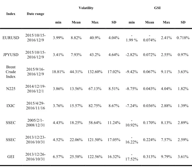
The basic statistics of calculated GSI with λ = 0.8 and volatility for different financial markets are reported in Appendix Table 1.2. In Greenwood and Shleifer (2014), for different data sources, their estimated results of λ are different, which ranges from 0.33 to 0.92. Of all the six samples, the empirical result for Gallup survey, which has the second largest sample size and the most significant result, seems to be the most reliable test result. So, we discuss the statistics of GSI with λ = 0.8 which approximates the result of the regression for Gallup survey.

From this table, we can see that, being used to measure how volatile the market is, the volatility index itself is very volatile. The minimum values of the estimated volatility of these indexes are all approximately equal to 4% (except for volatility of Brent Crude Index which reaches to 18.81%). Although the maximum values vary across different markets, they are all far beyond the minimum values. For EURUSD and JPYUSD, the maximum volatility is about 40%, ten times that of its minimum value, but for Brent Crude Index, GEI and SSEC in 20013 and 2016, the maximum volatility hovers to more than 120%, about 30 times bigger than its minimum value. This huge difference indicates that volatility can change very intensely, especially in Brent Crude

volatility fluctuation, is also much higher in Brent Crude Oil market and Chinses stock market than in other markets. Besides, the mean value of estimated volatility calculated by high frequency approach is smaller than the standard deviation of returns used in

Table 1.1. This result is similar to previous papers such as Liu and Tse (2012), Amsköld

(2011), as extreme returns are more stressed in standard deviation method (Masset 2011). Although the size is different, the order is same. Brent crude oil future market has the highest level of volatility, Chinese stock market is more volatile than other stock markets, and currency market is the most stable one. These statistics document that, Brent Crude Oil market and Chinese stock market present not only higher but also more instable volatility than other markets.

Although the standard deviation of Extrapolation belief index, GSI, is not high, its value can become very extreme. For instance, the max value of GSI for Chinese GEI index, is 9.79%, meaning extrapolative investors is so optimistic about future that they believe the price can still raise for about another ten percent. On the contrary, the minimum value of GSI for GEI index drops to -17.52%, indicating extrapolation belief make investors hold extreme pessimistic opinions about future returns. Besides, these severe preconceptions caused by extrapolation bias most occurred during the bubble period when volatility was also extremely high simultaneously.

Appendix Figure 1.3 is a demonstration of the fluctuation of volatility (blue line)

and the changing GSI (red line) while the black line means the GEI index. As shown in this picture, volatility starts to raise as the bubble grows since March 2015, and it continues raising even after the bubble busted. Eventually it reaches to its peak--more

than 120% on 9th July 2015, the most panicking time of the whole market. GSI, the extrapolation belief of individuals, also grows as the bubble generates like volatility index, showing the increasing enthusiasm of extrapolative investors. When the bubble begins to fall, GSI turns to negative as investors become pessimistic. It decreases to its minimum when the volatility reaches its peak. It seems the evolution of investors extrapolation belief, positive or negative, is associated with the evolution of volatility.

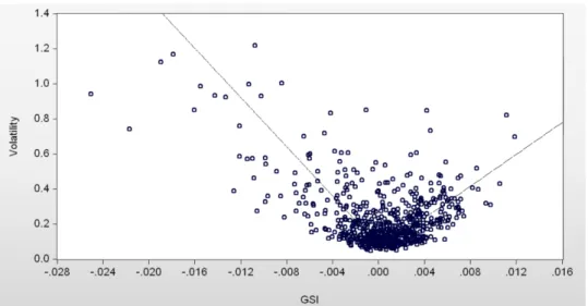
Appendix Figure 1.4, the scatterplot of volatility versus GSI for Chinese Growing

Enterprise stock market (GEI), gives a further demonstration of the contemporaneous GSI--volatility relationship. We can clearly see that, no matter positive or negative, the development of individuals’ extrapolation belief, measured by GSI, is associated with growing volatility.

Similar things happen to other two samples of Chinese stock market where distinguished bubble period can also be easily noticed, as shown in Appendix Figure

1.5 and Figure 1.6. Also, high volatility is accompanied by extreme values of GSI can

also be found in Japanese stock market, Nasdaq stock market and in Brent Crude oil market (seen Appendix Figure 1.7, Figure 1.8 and Figure 1.9).

From these figures, we could assume that volatility can be affected by the magnitude of GSI. Individuals’ extrapolative belief, positive and negative, can both lead volatility to increase. To empirically investigate this, we use the following regression form

where d_E and d_F are two dummy variables aiming to distinguish positive or negative regions of GSI. Results are shown in the following section.

1.4.3 Empirical Test Result and Comparison of different markets

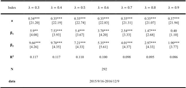
Firstly, as we don’t know exactly the weight that individual investors put into each past period, we calculate GSI with different values of λ ranging from 0.3 to 0.9, as suggested by Greenwood and Shleifer (2014). The results for different markets are listed in Appendix from Table 1.3 to Table 1.10.

As we see from these tables, the changing value of λ has little impact on the empirical test result. For example, for the currency market, for all the value of λ, all the empirical results for cE and cF are all insignificant. But for three samples of Chinese

stock market, although the size of estimated c_E and c_F are different with different value of λ, they are all highly significant. Besides, the R-squared value also changes limitedly. Similar things can also be found in Brent crude oil markets, the Japanese stock market as well as the Nasdaq stock market. Although the estimated c_E for Japanese stock market changes from weakly significant to insignificant as λ increases from 0.3 to 0.9, and the estimated c_E for Nasdaq stock is only insignificant when λ = 0.9, the estimated results don’t have a major difference with each other, as the significance of cF insists

for different λ, the R-squared value only has small changes. The estimated results don’t have major difference with each other.

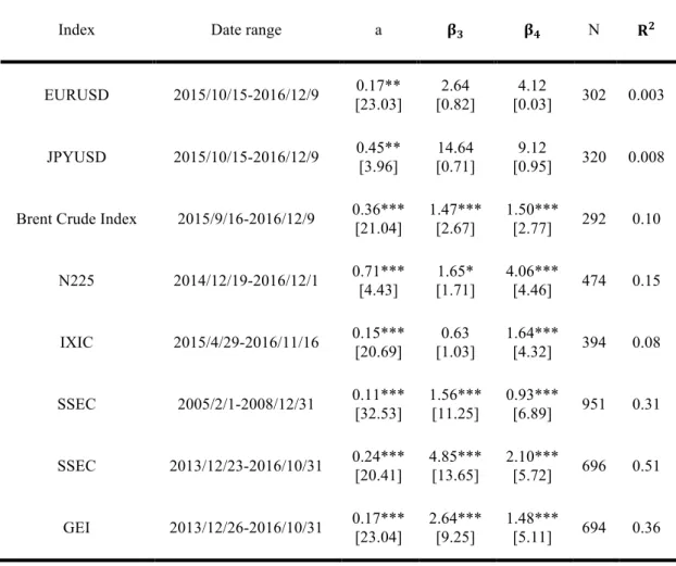
Therefore, for the convenience of comparison, the empirical results for different financial markets with λ = 0.8 are summarized in Appendix Table 1.11. Because

previous papers already show economic factors can partly explain the changes in volatility, we also introduce macro-economic factors into our regression to eliminate possible spurious regression as:

VolatilityL= a + βE∙ GSIL∙ DE GSIL> 0 + βF∙ GSIL ∙ DF GSIL≤ 0 + βn∙ oA+ uL (5)

where o_A means macro-economic factors. As we use daily data in our empirical test, the daily macro-economic factors are limited. Specifically, we use the Domestic Interbank Offered Interest Rate for the stock markets, and we use both countries’ Interbank Offered Rate for the currency market (although we only show the regression result with US. Interbank Offered Interest Rate). Because the Crude Oil Future is traded world-widely, we introduce the US Dollar Index as the explaining economic factor. All the empirical test results of regression form (5) for different financial markets are listed in Table 1.11 too.

Some meaningful conclusions can be established. Firstly, according to our empirical test result, GSI can significantly impact volatility in most of the financial markets. Moreover, it has much higher explaining power than economic factors. Particularly, as summarized in Table 1.11, cF is highly significant (P<0.01) for almost all the samples

(except for the currency markets). c_E is also highly significant for Chinses stock market samples. When we only use the economic factors as the explaining variable, the MF _is

quite small, which is consist with previous researcher’s’ finding that economic factors have little ability to explain the time varying volatility. On the contrary, if we use GSI as the explaining variable, MF _{increases significantly, indicating a much better}

regression result. More importantly, even if we include the macroeconomic factors in the regression, there is no significant change in the regression results. Taking Chinese GEI market for example, although the coefficient of Shibor is strictly positive, the R-squared value is only 0.12 when we only use Shibor as the explaining variable. But it increases to as much as 0.48 when we introduce GSI into the regression. Furthermore, if we introduce economic factors into equation (4), the significance of c_E and c_F insists, the R-squared value is similar as before. These significant results verify our assumption that volatility can be caused by individuals’ extrapolation belief.

Secondly, the significance level for different markets is different. For instance, Chinese stock market, where individual investors’ trading volume takes the biggest proportion, has the most significant regression results--both c_Eand c_F are significant at the 1% significance level. R-squared values also indicate GSI has the biggest explanatory power for volatility in Chinese stock market. With a size of 0.51, R-squared value for the second Chinese stock market sample (SSEC index from 2013/12/23 to 2016/10/13) implies a well-fitting regression. For other two Chinese stock market samples, R-squared values are both above 0.3, still bigger than other financial markets. As for Japan Stock market, Nasdaq stock market and Brent oil commodity future market, we only find less significant empirical regression results or a weaker explanatory power of GSI for volatility. Although c_F, the coefficient of the negative GSI, is highly significant (at the 1% significance level) for all these three markets, cE,

the coefficient for the positive GSI, performs much worse. It is only significant at the 5% significance level for Brent crude oil market and at the 10% significance level for

Japanese stock market while non-significant for Nasdaq stock market. Besides, R-squared values for these three markets are only about 0.1, which also suggest a weaker relation between GSI and volatility. For the currency markets, where individual investors take the minimum trading volume proportion, no significant regression result can be found. In a word, GSI has different ability to explain volatility in different financial markets.

Besides the diverse significant levels among different financial markets, the asymmetric GSI-Volatility relation is also proved. Our empirical results indicate c_F > c_E for all samples which have significant regression result. Besides magnitude, significant levels for these two coefficients are also different. For Japan Stock market, Brent oil commodity future market and Nasdaq stock market, c_F are all more significant than its counterpart, especially for the Nasdaq stock market, where the positive GSI cannot significantly affect volatility according to our empirical test.

Moreover, to formally test the asymmetric GSI-Volatility relation, we use the following regression form:

N^_`VU_UVaA = ` + cn #$%A + cp∙ #$%A ∙ dF #$%A ≤ 0 + gA (3.1.4)

in which we take c_F = c_E = c_n and c_p is insignificant as the null hypotheses. But according to our test result of 3.13 (represented in Table 1.12), c_p are significant for all the financial markets (except for the currency market). Also, for all the samples with the significant c_p, we can find c_p+ c_n = c_F, and c_E = c_n,which officially reject the

null hypotheses—there does exist an asymmetric GSI-Volatility relation in these financial markets.

This inequality reveals that negative GSI has stronger explanatory power to volatility than positive GSI. In other words, volatility is more easily affected by extrapolation belief in a declining market.

1.4.3 Result comparison of different stages

From the regression results of Table 1.11, we can find that when there is a bigger proportion of individual investors, there will be a more significant regression result. So, we could make the assumption that the effect extrapolation belief has on volatility is determined by the proportion of individual investors or the influence of individual investors to pricing. To further verify this assumption, this paper also compares different stages of the same market: bubble stages and other stages.

From Figure 1.3, Figure 1.5 and Figure 1.6 we can easily notice two bubble stages in Chinese stock market, the 2005-2008 stock bubble and 2015-2016 stock bubble. A financial bubble is often portrayed as the asset price rushes abnormally high compared with its fundamental value (Brunnermeier and Oehmke, 2012). As displayed in these figures, from 2013 to 2016, the SSEC index hovered to 5178 point followed by a big collapse of 50% within three months, while GEI index performs similarly by losing more than 56% in the same short time after its rising from around 1300 to a maximum of 4037 point. In both figures, volatility grows and fluctuates with bubble’s generation,

and become even higher and more fluctuant during bubble’ collapse. Similar things happen to SSEC index during 2005 and 2008.

Inexperienced individual investors are continually attracted to “gamble” in the market during the bubble periods. Kindleberger and Aliber (2005, p. 25) suggest that people who are indifferent to such investment are brought into the market. “Even chimney-sweeps and old clothes women dabbled in tulips.” as described by Mackay (1841). “Youth had taken over Wall Street.” happened during the stock market boom of the late 1960s (Brooks’ (1973, p. 211)). The same thing happens to Chinses stock market. Appendix Figure 1.10 shows the development of monthly new individual investors (blue line) and proportion of active account (red line) according to monthly reports of CSDC (China Securities Depository and Clearing Corporation) from 2014 Jan. to 2016 Nov., the second bubble period of Chinese stock market. Because individual investor’ accounts occupy about 99% of total accounts in Chinese stock market, the ups or downs of active account can be regards as the return or leave of individual investors who have already own a stock account. In this picture, we can feel the enthusiasm of new individual investors and the newfound interest of “old” individual investors when the price rises (black line in Figure 1.10), or the depression of individual investors as price falling. In a word, individual investors are much more active during bubbles. Hence, the correlation between volatility index and GSI should be bigger during bubbles.

To compare the different influence of extrapolation belief to volatility during different periods (bubbles period or non-bubble periods), each of the samples drawn

bubble stage and the non-core stage. The core-bubble stage is selected according to:(1) it should contain the most distinguished part of the bubble, i.e., the stage when the price reaches a very high level. (2) To avoid reliable test issues, the sample interval should not be too short. The rest time is the non-core stage. Even if we cannot calculate the fundamental value of each index, but based on the price level, we can at least distinguish when is bubble more severe. The core-bubble stage of each sample is represented by the green box in Figure 1.3, Figure 1.5 and Figure 1.6. The comparison result is reported in Appendix Table 1.13.

As represented in Table 1.13, empirical test result varies significantly across different stages. For all three samples, the least squares regression does perform better in core-bubble stages than in non-core stages. Especially for the latter two samples (from 2013 to 2016), after casting the most distinguished bubble stage, c_E, which is highly significant for the core-bubble stage and for the whole sample (see Table 2), only shows weak significance (at 10% level). R-squared value also drops to less than 0.1, which means the non-core stage of these two samples only have the similar performance with developed stock market and the Brent crude oil future market. Non-core stage of the third sample (SSEC 2005-2008) have a better regression result but it is still incomparable with the core-bubble stage. Besides the different regression significance between core-bubble stage and non-core stage, the asymmetric explanatory power of positive and negative GSI to volatility index is also reflected as cF > cE still holds for

These significant differences verify the conjecture that when the market has a bigger proportion of individual investors, the correlation between volatility index and individuals’ extrapolation belief should be higher. So, we may cautiously get the conclusion that individuals’ trading proportion is critical of explanatory power of GSI to volatility index. Therefore, extrapolation belief can be a reason that drives volatility to change, especially when individual investors have a large influence on pricing, like in Chinese stock market.

1.5 Further Discussion

To the author’s best knowledge, our paper is the first to use empirical test to investigate how individuals’ extrapolation belief can affect volatility across time. According to this paper’s result, extrapolation beliefs can not only cause the "excess volatility puzzle" as show in the existing papers, but also can drive volatility to vary over time. As discussed above, micro and macroeconomic variables can only partly explain why volatility changes across time (Bollerslev, Engle, and Wooldridge (1988), Schwert (1989)), so this approach offers a new method to study the variation of volatility.

Now the challenge is that existing theories about extrapolation are not enough for us to fully understand this relation between GSI and volatility. To further illustrator this, let’s assume the price follows the stochastic process as:

where R_A is the log value of current price, r_A stands for drift component of this process, i.e. the instantaneous conditional mean of return at time t, t is a standard Brownian motion while s_A represents a stochastic process independent of t_A , it also signifies the instantaneous volatility. Therefore, we can calculate the return as

@_AO = R_AO− R_AOST = AO r_Aq_A

AOST + sAqtA

AO

AOST (7)

and its quadratic variation QV(V_H, V_HGE) is

QV(V_H, V_HGE) = AO s_AF_qV

AOST (8)

Equation (8) shows that according to quadratic variation theory, innovations of the mean component r_A cannot change the variation of the return @_AO. Further, by semi-martingale theory, when the observation number increases, realized volatility will eventually become equivalent to the return quadratic variation QV (Protter 1990) :

MN_A = PQ @_A,HF

HDE → xNA= _AGEA sAFqA = sAF as ?A → ∞ (9)

Equation (9) proves the unbiasedness and accuracy of using Realized Volatility to estimate the instantaneous volatility. It also shows that r_A won’t affect instantaneous volatility estimated by high frequency Realized Volatility approach. But, the existing extrapolation theories all emphasize it is investor’s expectation of future returns that can be affected by past price changes. In most of these models, the equilibrium price is determined through the interaction between rational inverters’ expectation (which is determined by the stochastic information process), and extrapolative investors’ expectation which is only about past price changes. Therefore, according to previous

studies, we cannot connect the instantaneous volatility s_A with individuals’ extrapolation belief. Hence, why extrapolation belief can affect instantaneous volatility still needs theoretical explanations.

Although extrapolation is one of the most important biases individual are facing, it is not all of them. Overconfidence, for example, is another irrational belief individual may suffer. Overconfident means irrational traders are too “confident” about the accuracy of their private information signals (Gervais and Odean (2001)). Therefore, they usually ignore other investors’ trading behave when they make investment decisions. This bias can also generate several market anomalies, like the “excess volatility” puzzle and high trading volume (Odean 1998, Dumas, Kurshev and Uppal 2009), or even a sustainable bubble (Scheinkman and Wei Xiong 2003). Nevertheless, there is no foundational work as Greenwood and Shleifer (2014) about overconfidence, which can help to calculate how “overconfidence” individuals are.

Therefore, we currently may not be able to empirically study the effect of other individuals’ irrational beliefs on the fluctuation in volatility. We are hoping related works based on survey evidence or experimental evidence can emerge to help us with this dilemma. After all, it is not enough to study the aggregate market phenomenon with only one individual’s irrational bias.

1.6 REFERENCE

ABREU, D. & BRUNNERMEIER, M. K. 2003. Bubbles and crashes. Econometrica, 71, 173-204.

AMSKÖLD, D. 2011. A comparison between different volatility models.

ANDERSEN, T. G. & BOLLERSLEV, T. 1998. Answering the skeptics: Yes, standard volatility models do provide accurate forecasts. International economic review, 885-905.

ANDERSEN, T. G., BOLLERSLEV, T., DIEBOLD, F. X. & EBENS, H. 2001. The distribution of realized stock return volatility. Journal of financial economics, 61, 43-76.

ANDERSEN, T. G., BOLLERSLEV, T., DIEBOLD, F. X. & LABYS, P. 2003. Modeling and forecasting realized volatility. Econometrica, 71, 579-625.

ANDERSEN, T. G., BOLLERSLEV, T., DIEBOLD, F. X. & VEGA, C. 2003. Micro effects of macro announcements: Real-time price discovery in foreign exchange.

American Economic Review, 93, 38-62.

BALFOUR, N. & MACKAY, S. 1980. Paul of Yugoslavia: Britain's maligned friend, H. Hamilton.

BARBERIS, N., GREENWOOD, R., JIN, L. & SHLEIFER, A. 2015. X-CAPM: An extrapolative capital asset pricing model. Journal of financial economics, 115, 1-24. BARBERIS, N., GREENWOOD, R., JIN, L. & SHLEIFER, A. 2016. Extrapolation

BARBERIS, N., HUANG, M. & SANTOS, T. 2001. Prospect theory and asset prices.

The quarterly journal of economics, 116, 1-53.

BARBERIS, N. & SHLEIFER, A. 2003. Style investing. Journal of financial

Economics, 68, 161-199.

BARBERIS, N., SHLEIFER, A. & VISHNY, R. 1998. A model of investor sentiment1.

Journal of financial economics, 49, 307-343.

BARBERIS, N. & THALER, R. 2003. A survey of behavioral finance. Handbook of

the Economics of Finance, 1, 1053-1128.

BARNDORFF-NIELSEN, O. E. & SHEPHARD, N. 2001. Modelling by Lévy processess for financial econometrics. Lévy processes. Springer.

BARNDORFF-NIELSEN, O. E. & SHEPHARD, N. 2002. Estimating quadratic variation using realized variance. Journal of Applied econometrics, 17, 457-477. BLACK, F. 1992. Beta and return. Journal of portfolio management, 1.

BOLLERSLEV, T., ENGLE, R. F. & WOOLDRIDGE, J. M. 1988. A capital asset pricing model with time-varying covariances. Journal of political Economy, 96, 116-131.

BRENNAN, M. J. 2004. How did it happen? Economic Notes, 33, 3-22. BROOKS, J. 1973. The Go-go Years, Weybright and Talley.

BRUNNERMEIER, M. K. & OEHMKE, M. 2013. Bubbles, financial crises, and systemic risk. Handbook of the Economics of Finance. Elsevier.

CASTANIAS, R. P. 1979. Macroinformation and the variability of stock market prices.

The Journal of Finance, 34, 439-450.

CHARLES, M. 1841. Extraordinary popular delusions and the madness of crowds.

Radford, VA: Wilder.

CHRISTIANSEN, C., SCHMELING, M. & SCHRIMPF, A. 2012. A comprehensive look at financial volatility prediction by economic variables. Journal of Applied

Econometrics, 27, 956-977.

CUTLER, D. M., POTERBA, J. M., SHEINER, L. M., SUMMERS, L. H. & AKERLOF, G. A. 1990. An aging society: opportunity or challenge? Brookings

papers on economic activity, 1990, 1-73.

CUTLER, D. M., POTERBA, J. M. & SUMMERS, L. H. 1990. Speculative dynamics and the role of feedback traders. National Bureau of Economic Research.

DE BONDT, W. F. 1998. A portrait of the individual investor. European economic

review, 42, 831-844.

DE LONG, J. B., SHLEIFER, A., SUMMERS, L. H. & WALDMANN, R. J. 1990. Noise trader risk in financial markets. Journal of political Economy, 98, 703-738. DE LONG, J. B., SHLEIFER, A., SUMMERS, L. H. & WALDMANN, R. J. 1990.

Positive feedback investment strategies and destabilizing rational speculation. the

Journal of Finance, 45, 379-395.

DUMAS, B., KURSHEV, A. & UPPAL, R. 2009. Equilibrium portfolio strategies in the presence of sentiment risk and excess volatility. The Journal of Finance, 64, 579-629.

ENGLE, R. F. & RANGEL, J. G. 2008. The spline-GARCH model for low-frequency volatility and its global macroeconomic causes. The Review of Financial Studies, 21, 1187-1222.

EUN, C. S. & HUANG, W. 2007. Asset pricing in China's domestic stock markets: Is there a logic? Pacific-Basin Finance Journal, 15, 452-480.

FAMA, E. F. 1965. The behavior of stock-market prices. The journal of Business, 38, 34-105.

FLANNERY, M. J. & PROTOPAPADAKIS, A. A. 2002. Macroeconomic factors do influence aggregate stock returns. The review of financial studies, 15, 751-782. FLEMING, M. J. & REMOLONA, E. M. 1999. Price formation and liquidity in the US

Treasury market: The response to public information. The journal of Finance, 54, 1901-1915.

GERVAIS, S. & ODEAN, T. 2001. Learning to be overconfident. the Review of

financial studies, 14, 1-27.

GILCHRIST, S., HIMMELBERG, C. P. & HUBERMAN, G. 2005. Do stock price bubbles influence corporate investment? Journal of Monetary Economics, 52, 805-827.

GILOVICH, T., VALLONE, R. & TVERSKY, A. 1985. The hot hand in basketball: On the misperception of random sequences. Cognitive psychology, 17, 295-314. GREENWOOD, R. & SHLEIFER, A. 2014. Expectations of returns and expected

Finance, 56, 1533-1597.

HONG, H. & STEIN, J. C. 1999. A unified theory of underreaction, momentum trading, and overreaction in asset markets. The Journal of finance, 54, 2143-2184.

HONG, H. & STEIN, J. C. 2007. Disagreement and the stock market. Journal of

Economic perspectives, 21, 109-128.

HUBERMAN, G. 2005. A simple approach to arbitrage pricing theory. Theory of

Valuation. World Scientific.

K BRUNNERMEIER, M. & NAGEL, S. 2004. Hedge funds and the technology bubble.

The Journal of Finance, 59, 2013-2040.

KINDLEBERGER, C. P. & ALIBER, R. Z. 2000. Manias, panics, and crashes: a history of financial crises. The Scriblerian and the Kit-Cats, 32, 379.

KRISTOUFEK, L. & VOSVRDA, M. 2016. Gold, currencies and market efficiency.

Physica A: Statistical Mechanics and its Applications, 449, 27-34.

KYLE, A. S. 1985. Continuous auctions and insider trading. Econometrica: Journal of

the Econometric Society, 1315-1335.

LEROY, S. F. & PORTER, R. D. 1981. Stock price volatility: tests based on implied variance bounds. Econometrica, 49, 113.

LIU, X. F. & TSE, C. K. 2012. A complex network perspective of world stock markets: synchronization and volatility. International Journal of Bifurcation and Chaos, 22, 1250142.

MACKAY, C. 2015. Extraordinary popular delusions, Templeton Foundation Press. MCALEER, M. & MEDEIROS, M. C. 2008. Realized volatility: A review.

Econometric Reviews, 27, 10-45.

MENGEL, F. & SCIUBBA, E. 2010. Extrapolation and structural learning in games.

Maastricht University and Birkbeck College London.

MITTNIK, S., ROBINZONOV, N. & SPINDLER, M. 2015. Stock market volatility: identifying major drivers and the Nature of Their Impact. Journal of Banking &

Finance, 58, 1-14.

ODEAN, T. 1998. Volume, volatility, price, and profit when all traders are above average. The Journal of Finance, 53, 1887-1934.

ODEAN, T. 1998. Are investors reluctant to realize their losses? The Journal of finance, 53, 1775-1798.

OFFICER, R. R. 1973. The variability of the market factor of the New York Stock Exchange. The Journal of Business, 46, 434-453.

SCHEINKMAN, J. A. & XIONG, W. 2003. Overconfidence and speculative bubbles.

Journal of political Economy, 111, 1183-1220.

SCHWERT, G. W. 1989. Why does stock market volatility change over time? The

journal of finance, 44, 1115-1153.

SHEFRIN, H. M. & THALER, R. H. 2004. Mental accounting, saving, and self-control.

Advances in behavioral economics, 395-428.

SHILLER, R. J. 1980. Do stock prices move too much to be justified by subsequent changes in dividends? : National Bureau of Economic Research Cambridge, Mass., USA.

Princeton university press.

STOLL, H. R. & WHALEY, R. E. 2010. Commodity index investing: speculation or diversification?

STRAHILEVITZ, M. A., ODEAN, T. & BARBER, B. M. 2011. Once burned, twice shy: How naïve learning, counterfactuals, and regret affect the repurchase of stocks previously sold. Journal of Marketing Research, 48, S102-S120.

WEST, K. D. 1988. Dividend innovations and stock price volatility. Econometrica:

Appendix 1

Figure 1.2 Realized volatility of Brent Crude oil index

Calculation method: 30 days rolling windows of historical realized volatility Source: Yahoo finance

Figure 1.3 GSI and volatility index in Shenzhen Growth Enterprise stock market We present its absolute value of GSI, which is computed according to Greenwood and Shleifer (2014), with red line (red axis)

while red-dot line shows its negative values. The blue line denotes volatility index estimated by high frequency realized volatility approach (blue axis). Black line (black axis) represents IXIC, the index of Nasdaq stock market.

Figure 1.4 Scatterplot of GSI versus volatility index for GEI

Figure 1.5 GSI and volatility index in Shanghai mainboard stock market (2005 -2008) We present its absolute value of GSI, which is computed according to Greenwood and Shleifer (2014), with red line (red axis)

while red-dot line shows its negative values. The blue line denotes volatility index estimated by high frequency realized volatility