リーゼガング現象の数理的様相 (反応拡散系におけるパターン形成と漸近的幾何構造の研究)

(1)

A

_Mathematical

Aspect

for

Liesegang

_Phenomena

-

リーセガング現象の数理的様相

-広島大学大学院理学研究科

(

数理分子

)

大酉勇 (Isamu Ohnishi)*

Department

of

Mathematical

and Life Sciences,

Graduate School

of Science,

Hiroshima

University

1 Liesegang

Phenomena

Liesegang phenomenon is pattern

formation

appeared in

a

gel-containingsystem [1]. We

can

observe striped patterns like in Fig.1, 2, especially in the presence _{of concentration}

gradients in initial data. These striped patterns

are

called “the Liesegang band” and “the

Liesegang ring” respectively, because they

_were

discovered by R. E. Liesegang in

1896

for

the first time. In this paper,

we

discuss about the mechanismof thiskind ofstripedpattern

formation.

The Liesegang band is

obtained

,

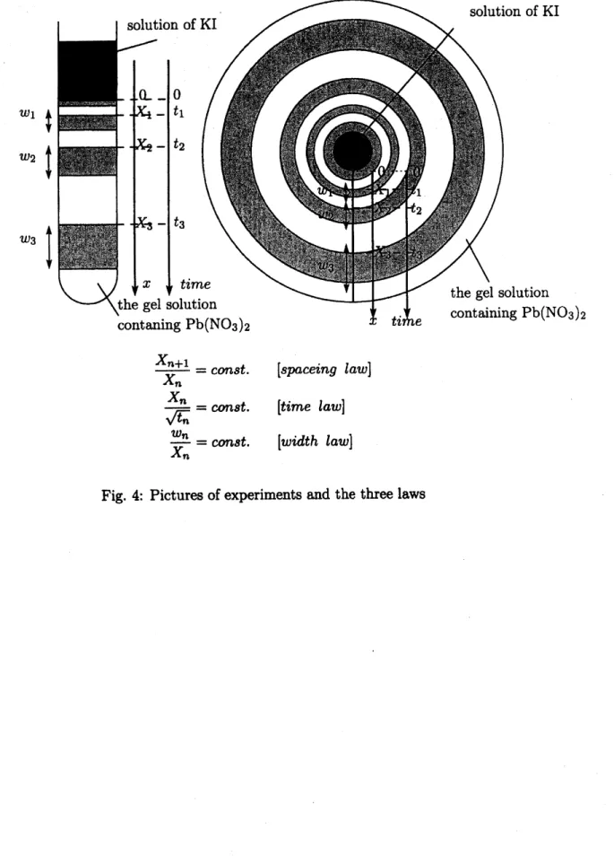
$\mathrm{b}\mathrm{y}$, forexample, thefollowingprocedure. A

$\mathrm{s}$ lution of

one

soluble electrolyte, for instance, lead

nitorate

$(\mathrm{P}\mathrm{b}(\mathrm{N}\mathrm{O}_{3})_{2})$, at relatively low concentration

is placed in

a test

tube to which

a

gel-forming material is added. After

a

gel is formed,

another electrolyte solution, such

as

the potasium iodide (KI), normally at substantially

higher concentration, ispoured

on

thetop ofthegel containing Pb(NOs)2. The iodide

ons

$(\mathrm{I}^{-})$ diffuse into the gel and react with

lead ions $(\mathrm{P}\mathrm{b}^{+})$ to form lead iodide

$(\mathrm{P}\mathrm{b}\mathrm{I}_{2})$ which is

almost insoluble.

$\mathrm{P}\mathrm{b}^{2+}+2\mathrm{I}^{-}arrow \mathrm{P}\mathrm{b}\mathrm{I}_{2}$

After

an

interval of

minutes

there appear bands, s0-called the Liesegang band like

a

Fig. 1.

The times after the start of the experiment at which pictures (a) to (c)

were

taken,

are as

follows: (a)

2

hours, (b) 8 hours, and (c)

48 hours.

.

_{この論文は、広島大学大学院理学研究科の三村昌泰教授、およひ、}_{同研究科の大学院生てあった濱岡玉緒氏と}

の共同研究てす。

(2)

We

can

make the Liesegang ring similarly. A solution ofKI is set up in theinner part of

a

petri dish whose outer part is occupied by Pb(NOs)2 contained in gel. Here, KI solution

is much higher concentration than $\mathrm{P}\mathrm{b}(\mathrm{N}\mathrm{O}_{3})_{2}$

.

As $\mathrm{I}^{-}$ diffuse into

an

outer solution, the insoluble salt $\mathrm{P}\mathrm{b}\mathrm{I}_{2}$ precipitates and rings, s0-called the Liesegang ring appear like

a

Fig.2.

It is also well-known that these striped patterns satisfy three periodic laws, spacing law,

time law, and width law inchemicalexperiments practically [5]. spacing law

can

bedescribed

as

$X_{N+1}=pXn,$ where $X_{N}$ is the

distance

of$N$-th band (ring) location from

an

original

junction and $p$ is

a

positive constant (Fig.3). time law and width law

are

expressed

as

$\sqrt{t_{N}}=qX_{N}$ and $w_{N}=rX_{N}$ respectively, where $t_{N}$, $w_{N}$, $\mathrm{q}$and $\mathrm{r}$

are

the interval from time

when the experiment started to formation time ofthe $N$-th band (ring), width of the $\mathrm{i}\mathrm{V}$-th

band (ring) and positive constants.

There

are a

lot ofmathematical modelsknown,whichdescribes theinterestingphenomena.

We adopt the reduced KR model which is reduced from the well-known Keller-Rubinow

model. We

can

referto the forthcomingpaper [2] about thedetailof theKR model and the

(3)

Fig. 1: the Liesegang band [3] Fig. 2: the Liesegang ring [4]

(4)

$\frac{X_{n+1}}{X_{n}}=cnst$

.

$\frac{X_{n}}{\sqrt{t_{n}}}=$const. $\frac{w_{\hslash}}{X_{n}}=$const. [spaceing law] [time law] [width law]

(5)

2 Mathematically

_{rigorous Analysis for the reduced}

_KR

_model

2.1

Existence

of

a

time

local weak solution

Without loss of generality,

we

make $D_{c}=1$

as we

change the reduced KR model to _the

dimension less form.

$\{$

$c_{t}=\Delta c+b_{0}S’(t)\delta(r- 5(t))$ $-qP(\mathrm{c}, d)$,

$0<t<T$

, $\mathrm{x}$ $\in \mathrm{R}^{n}$,

$d_{t}=qP(c,d)$,

_$0<t<T$

_, $\mathrm{x}$ $\in \mathrm{R}^{n}$,

$(B.C.)$ $\lim_{farrow\infty}c(t,\mathrm{x})=0,$ $0<t<T,$

$(I.C.)c(0, \mathrm{x})=0,$ $d$(0,x) _$=0,$ $\mathrm{x}\in \mathrm{R}^{n}$,

(2.1)

where

$\delta$

means

the

Dirac

$\delta$ in

one

space dimension,

$P(c, d)=\{$ $(c-C_{a})+$,

on

{

$\mathrm{x}\in \mathrm{R}^{n};c>C_{s}$

or

$d>0$

}

$,$

0, otherwise,

$q>0$, $b_{0}>0$, $C_{s}\geq C_{a}\geq 0$ : given constants,

$S(t)=\alpha\sqrt{t}(\alpha>0)$ : given function.

$r$ is definedby

$r=||=$ $x_{n-1}^{2}+x_{2}^{2}+\cdots+xB,$ $\mathrm{x}=$ $(x_{1}, x_{2}, \cdot\cdot| , x_{n})\in \mathrm{R}^{n}$

.

In this chapter

we

consider (2.1) in

case

of$C_{a}=0.$

We first define

a

weak solution of (2.1). Let $c(\cdot, \cdot)\in L^{1}(0, T;W^{1,\infty}(\mathrm{R}^{n}))$, $d(\cdot, \cdot)\in$

$L^{\infty}$_{$((0, 7 )$} $\mathrm{x}\mathrm{R}^{n})$

.

Ifthese satisfy

$c(t, \mathrm{x})$ $=$ $\int_{0}^{t}\int_{\mathrm{R}^{n}}\frac{1}{(4\pi(t-s))^{\frac{n}{2}}}e^{-\frac{\{\mathrm{x}-\xi)^{2}}{4(t-\epsilon)}}b_{0}S’(s)\delta(\lambda-S(s))$th_$ds$

$-q \int_{0}^{t}\int_{\mathrm{R}^{n}}\frac{1}{(4\pi(t-s))^{\frac{n}{2}}}e^{-\frac{(\mathrm{x}-\xi)^{2}}{4(t-s)}}P(c,d)d\xi ds$, (2.2) $d(t, \mathrm{x})$ $=$ $q \int_{0}^{t}P(c, d)$ds,

then

we

call

a

couple ofthem

a

weak solution of (2.1), where

we

define

A by

$\lambda=|4|=\sqrt{\xi_{1}^{2}+\xi_{2}^{2}+\cdots+\xi_{n}^{2}}$,

for$4=$ $(\xi_{1}, \cdots,\xi_{n})\in \mathrm{R}^{n}$

.

Weadopt the folowing form of the polar coordinate in $\mathrm{R}^{n}$ to rewrite (2.2):

$\{$

$\xi_{1}$ $=$ A$\sin\beta_{n-1}\sin\sqrt n-2\ldots\sin\sqrt 2\cos\beta 1$

,

$\xi_{2}$ $=$ A $\sin\sqrt n-1\sin\beta_{n-2}\ldots\sin\sqrt 2\sin\beta_{1}$,

.

$\cdot$

.

$\xi_{n}$ _$=$ A_{$\cos\sqrt n-1$},

(6)

6

$0\leq\lambda<\infty$

,

$0\leq$ $\mathrm{f}1_{1}$ $<2\pi,$

$0\leq\beta_{j}<\pi(j=2,3, \cdot\cdot \mathrm{L}, n-1)$

.

Therewritten formof (2.2) is

$c(t,\mathrm{x})$ $=$ $\int_{0}^{t}\int_{\mathrm{R}^{n}}\frac{1}{(4\pi(t-s))^{n}\tau}e^{-\frac{(\mathrm{x}-\xi(\lambda))^{2}}{4(l-\epsilon)}}b_{0}S’(s)\delta(\lambda-S(s))J(\lambda,\beta)d\lambda d\beta ds$ ,

$-q$$\int_{0}^{t}7_{n}\frac{1}{(4\pi(t-s))^{\frac{n}{2}}}e^{-\frac{(\mathrm{x}-\epsilon(\lambda)\}^{2}}{4(t-s)}}P$(c,$d$)$J(\lambda, \mathrm{B})$ $d\lambda d\beta ds$, (2.4)

where $\beta=$ $(\beta_{1}, \cdots, \mathrm{j}3_{n-1})$, $d\beta=d\beta_{1}\ldots$$d\beta_{n-1}$

,

and

$J(\lambda, \beta)=2^{n-1}\sin^{n-2}\beta_{n-1}\sin^{n-3}\beta_{n-2}\cdots\sin \mathrm{f}1_{2}$

is the Jacobian of the polar coordinates, and $\xi(\lambda)(= (\xi_{1}(\lambda), \xi_{2}(\lambda)$,$\cdots$ ,$\xi_{n}(\lambda)))$

means

the

variableschanged by

use

of(2.3). Weemphasize the dependency onlyuponA because there

is the term ofthe Dirac $\delta$

on

A in the first term ofthe right-hand side of (2.4).

We remark that, if$n=1$ and the boundary condition of$c$ at $x=0$ is the homogeneous

Neumann, the corresponding integral equation of$c$is

$c(t, x)$ $=$ $\int_{0}^{t}\frac{b_{0}S’(s)}{\sqrt{4\pi(t-s)}}(e^{-\frac{(\alpha-S(s))^{2}}{4(t-\epsilon)}}+e^{-\frac{(oe+S(s))^{2}}{4(l-s)}})ds$

$-q$$\int_{0}^{t}\int_{0}$

”

$\frac{1}{\sqrt{4\pi(t-s)}}(e^{-\mu_{\mathrm{t}-s)}^{2}}\emptyset-+e^{-\frac{(x+\xi)^{2}}{4(t-s)}})P(c,d)d\xi ds$

.

Therefore

we

shouldalso definetheweak solution separately in

one

space deimension by

use

of the above expression. But the mathematical argument in this chapter is appricable to

the

case

of

one

space dimension.

We define the operator $G$ by

$G(c)=$ (theright-hand side of (2.4))

and the space of functions $K$ by

$K=L^{1}(0,T;L^{\infty}(\mathrm{R}^{n}))$

.

Let

us

define the

norm

of$K$ by

$||c||_{K}=/_{0}^{T}||c(t, \cdot)$$||L\infty dt$,

and $K$ is a Banach space. We note that $G$ is

a

compact operator

on

$K$ for any $d(\cdot, \cdot)\in$

$L^{\infty}$((0,i) $\mathrm{x}\mathrm{R}^{n}$), and note that let

us

$K_{1}=\{c\in K;||c||_{K}\leq 1\}$,

(7)

Theorem 2.1 (existence _of_{a time local weak} _solution)

_If

_T $>0$ is smallsufficiently,

there exists a weak solution

_of

(2.1) such that c $\in K$ and d$\in L^{\infty}((0,$T) $\cross$ Rn). $\mathrm{p}\mathrm{r}.)$ We first note that, for any$c\in K$,

$d(t, \mathrm{x})(0<t<T)$ satisfies

$d(t,\mathrm{x})$ $=$ $q \int_{0}^{t}P(c, d)ds$

$=$ $\{$

$q \int_{0}^{t}c(s, \mathrm{x})ds$, if_{$c>C_{s}$} or _$d>0,$

0, otherwise, (2.5)

and $d(\cdot, \cdot)\in L^{\infty}((0, T)\mathrm{x}\mathrm{R}^{n})$

. Therefore

we

regard $d$

as

a function

of $c$

.

If

we

put the

function $d(c)$ into $P(c, d)$ of (2.2), then we _{consider of (2.2)}

_as

_only $c$’s equation. We will

prove the existence of

a

solution $c\in K$ of _(2.2). _Let

us

_decide $d$ by

use

of (2.5) for _$c$

constructed already, and

we can

make

a

weak solution of (2.1) eventually.

Now

we

will estimete (2.4) for

any

$c\in K.$

[Estimate _{for the first} _term _{of the right-hand side of (2.4)]}

Let

us

makethefollowingchange ofvariables tothe first term of the right-hand side of(2.4),

$\{$

$p^{2}$ _$=$ $\frac{\mathit{8}}{t}$

,

(2.6) $x_{i}$ $=$ $S(t)y_{\dot{l}}$ $(i=1,2, \cdots, n)$,

and

we

get

$=$ _(2.7)

where $\mathrm{y}=$ $(y1,12, \cdots, y_{n})$ and $\mathrm{S}^{n-1}$

means

the unit sphere in $(\mathrm{v}\mathrm{z} ・1)$ space dimensions.

Theright-hand sideof (2.7) isindependent from$t$, and

moreover

it takes

a

boudedvalue at

$\mathrm{y}=(0, 0, \cdots, 0)$ and

converges

to

0 as

$|\mathrm{y}|arrow\infty$

.

Therefore it takes

a

positive maximumi

$\mathrm{n}$

Rn. There

exists

a

positive _constant $M_{1}$ independentof both $t$ and$\mathrm{x}$ such that

$|$the first term oftheright-hand side of

(2.4)$]$ $\leq M_{1}$

.

(2.8)

Thus

we

get

$\int_{0}^{T}||$the first term

(8)

8

[Estimate _{for the} $\mathrm{x}$-derivative of the first term of the right-hand side of (2.4)]

Let

us

notethat

$\frac{\partial}{\partial x_{\dot{l}}}=\frac{1}{S(t)}\frac{\partial}{\partial y_{i}}$ $(i=1,2, \cdots, n)$,

and

$\ovalbox{\tt\small REJECT}$

Therefore there exists

a

positive constant M2 such that

$|\mathrm{x}$ -derivative of the first term of

the

right-hand side of (2.4)|

$\leq M_{2}\sqrt{\frac{1}{t}}$

.

For any $7=2,3$,$\cdot\cdot$

.

,$n$, let

us

estimate $x_{j}$-derivative in the

same

manner, and there exists

a

positive constant $M_{3}$ independent ofboth $t$ and $\mathrm{x}$ such that

$|$the$\mathrm{x}$-derivative ofthe first termofthe right-hand side of$(2.4)|\leq nM_{2}\sqrt{\frac{1}{t}}$

.

Thus

we

get

$\int_{0}^{T}||\mathrm{x}$-derivative of the first termof the right-hand side of $(2.4)||_{L}\infty dt\leq 2nM_{2}\sqrt{T}r$

[Estimate_{for the second term of}the right-hand side of(2.4)]

$| \int_{0}^{t}\int_{\mathrm{R}^{n}}\frac{1}{(4\pi(t-s))^{\frac{n}{2}}}e^{-\frac{(\mathrm{x}-\xi(\lambda))^{2}}{4(t-*)}}P(c,d)J(\lambda,\beta)d\lambda d\beta ds|$

$\leq\int_{0}^{t}\int_{\mathrm{R}^{n}}\frac{1}{(4\pi(t-s))^{\frac{n}{2}}}e^{-\xi_{t-}^{\mathrm{x}}}\neq-*\neq^{2}d\xi||c(s, \cdot)||_{L}\infty ds$

.

(2.9)

Let

us

remark that

$\int_{\mathrm{R}^{n}}\frac{1}{(4\pi(t-s))^{\frac{n}{2}}}e^{-\frac{(\mathrm{x}-\xi)^{2}}{4(t-\epsilon)}}d\xi=1,$

and

we

get

(the right-hand sideof (2.9)) $=lt$$||c(s$

,

$\cdot$$)||\mathrm{z}\infty ds\leq||c||K$

.

Therefore

$\int_{0}^{T}$ (theleft-hand side of (2.9))$dt\leq||c||K$ $7_{0}^{dt=}T||c||_{K}T$

.

(9)

9

$| \frac{\partial}{\partial x_{1}}\int_{0}^{t}\int_{\mathrm{R}^{\hslash}}\frac{1}{(4\pi(t-s))^{\frac{n}{2}}}e^{-\frac{(\mathrm{x}-\xi(\lambda))^{2}}{4(t-s)}}P(c, d)J(\lambda, \beta)d\lambda d\beta ds|$

$\leq$ $\int_{0}^{t}(|\int_{x_{1}}^{\infty}\frac{1}{2\sqrt{\pi(t-s)}}(-\frac{x_{1}-\xi_{1}}{4(t-s)})e^{-\neg}4(t-s(x-\xi)^{2}$

,

$|$

$+| \int_{-\infty}^{x_{1}}\frac{1}{2\sqrt{\pi(t-s)}}(-\frac{x_{1}-\xi_{1}}{4(t-s)})e^{-\dashv_{4}^{-}+)^{2}}‘-*d\xi_{1}|(oe)$

$\int_{\mathrm{R}^{n-1}}\frac{1}{(4\pi(t-s))^{\frac{n-1}{2}}}e^{-\frac{\Sigma_{\dot{\mathrm{z}}=2}^{n}(x_{j}-\xi_{j})^{2}}{4(t-e)}}d\xi_{2}\cdots d\xi_{n}||c(s, \cdot)||_{L\infty}ds$

.

(2.10)

Let

us

make the following chenge of variable

$\theta_{1}=-\frac{x_{1}-\xi_{1}}{2\sqrt{t-s}}$, and $\int_{x_{1}}^{\infty}\frac{-(x_{1}-\xi_{1})}{8\sqrt{\pi}(t-s)^{\frac{3}{2}}}e^{-\frac{(oe-\xi)^{2}}{4(\ell-s)}}d\xi_{1}$ $=$ $\frac{1}{2\sqrt{\pi(t-s)}}7^{\theta_{1}e^{-\theta_{1d\theta_{1}}^{2}}}\infty)$ 1 $=$ $\overline{4\sqrt{\pi(t-s)}}$

.

Let

us

estimate the integral term

on

$(-\mathrm{o}\mathrm{o}, x_{1})$ in the

same

way

as

above, and note that $\int_{\mathrm{R}^{n-1}}\frac{1}{(4\pi(t-s))^{\frac{\mathfrak{n}-1}{2}}}e^{-\frac{\Sigma_{\mathrm{j}=2}^{n}(x_{\mathrm{j}}-\xi_{j})^{2}}{4(\mathrm{t}-s)}}d\xi_{2}\cdots d\xi_{n}=1,$

and

(the right-hand side of (2.10)) $= \int_{0}^{t}\frac{1}{2\sqrt{\pi(t-s)}}||c(s$,$\cdot$_$)||L\infty$ds.

Therefore

$\int_{0}^{T}$(theleft-hand side of (2.10))dt $\leq$

$\leq$

For any$j=2,3$,$\cdot\cdot$

.

(10)

io

Therefore, if$T>0$ issmall sufficiently, then for any $c\in K_{1}(\subset K)$

$||G(c]|K$ $\leq M_{1}T+nM_{2^{\sqrt{T}+}}(T+n\mathrm{a})$ $||c||K$

$\leq$ 1.

Thus $G$ is a compact operator from $K_{1}$ into $K_{1}$

.

By

we

of the Schauder’s fixed point

theorem,

we

conclude that there exists$c\in K_{1}$ such that $c=G(c)$

.

$\square$

Remark 2.2 We

see

thesolution

c

be bounded in $W^{1,\infty}(\mathrm{R}^{n})$ uniformly in time except the

time point t$=0$from the above proof.

2.2 Time global

solution

and its

regularity

Theweak solution satisfies the following:

$\mathrm{o}$ ‘Gap’ in time

occurs

at the moment when $t$ becomes positive in the meaningof $\sup-$

norm

because of the non-homogeneous term of the Dirac $\delta$

.

But the solution is

Lips-chitz continuous intime if$t>0.$

’ We cannot expect that the solution

on

$r=S(t)$ is smoother than in $W^{1}$,”(R$n$

), although it issmooth in $r\neq$S(t)

In fact, let

us

calculate it directly by

use

of (2.4), and if the solution exists

on

a time

interval $(0, 7 )$ for

some

positive constant $T$, it is Lipschitz continuous in

$0<t<T$

and is

in $C^{2}(\mathrm{R}^{\hslash \mathrm{S}}\partial D_{S(t)})$

,

and

moreover

$c\in L^{1}(0,T;W^{1,\infty}(\mathrm{R}^{n})\cap L^{p}(\mathrm{R}^{n}))$ $(1 \leq p\leq\infty)$

.

Here $D_{a}=\{\mathrm{x}\in \mathrm{R}^{n};|\mathrm{x}|<a\}$ for

any

$a>0.$

Next,

we

will prove that

a

time global solution exists. If $c\equiv 0,$ then the following

differencial inequality holds:

$\{$

$c_{t}\leq$ bc$+$

boS’{t)6(t

$-S(t)$) $-qP(c, d)$

$\lim_{farrow\infty}c(t,\mathrm{x})=0$ $c(0,\mathrm{x})=0.$

Therefore,

as

long

as

it exists, thesolutionof (2.4) satisfies

$c(t,\mathrm{x})\geq 0.$

We

see

precipitation

occur

continuouslyin

space

and time, if$C_{s}=C_{a}=0.$

We estimate

on

thesecondtermofthe right-hand side of (2.4).

(11)

1

$[$

As (2.7) and (2.8)

_are

_taken _into account,

$0\leq$ $c(t, \mathrm{x})$ $\leq$ $\int_{0}^{1}\int_{\mathrm{S}^{n-1}}\frac{b_{0}\alpha^{n}}{(4\pi(1-p^{2}))^{\frac{n}{2}}}e^{-\frac{\alpha^{2}(\mathrm{y}-\xi(\mathrm{p}))^{2}}{4(1-\mathrm{p}^{2})}}J(p, \beta)d\beta dp$ $\leq$ $M_{1}$,

(2.11) uniformly for $\mathrm{x}$

.

Therefore for any $T>0,$

$\int_{0}^{T}||c(t, \cdot)||L\infty dt\leq M_{1}T$

(2.12)

We estimate

on

$c_{\mathrm{x}}(t,\mathrm{x})$ in the

same manner

as

in the proof

of Theorem 2.1. In fact,

we

make the

same

calculation

as

in [Estimatefor the$\mathrm{x}$-derivative of the first term ofthe

right-hand side of (2.4)$]$ and [Estimate for the

$\mathrm{x}$-derivative of the second term of the right-hand

side of (2.4)$]$, and

we use

(2.11)

on

the way. Therefore there exists

a

positive consta $\mathrm{t}$ _{$M_{3}$} such that, for $i=1,$2,$\cdot\cdot 1$ ,_$n$,

$\int_{0}^{T}||c_{x_{i}}(t,\mathrm{x})||L\infty\leq M_{3}\sqrt{T}$

.

(2.13)

Thusthere exists

a

positive constant $M_{4}$ such that for any fixed $T>0$

$||c||_{K}\leq M_{4}(\sqrt{T}+T)$, _(2.14)

by

use

of (2.12) and (2.13).

Prom

(2.14)

_{we see}

the

solution

be in

a

bounded set for any

T $>0.$ This

means

that a_{time global solution exists.}

Remark 2.3 In the end ofthe section 2.2,

we

consider about radially symmetric solutions

of (2.1). If it is assumed that thesolution_{of (2.1) is radially symmetric, then it satisfies the}

equationsof the radially symmetric problem:

$\{$

$d_{t}=qP(cc_{t}=c_{\mathrm{r}r}+, \frac{n-1}{d)\mathrm{r}},c_{f}+b_{0}S’(t)\delta(r-S(t))-qP(c, d)$,

$(B.C.)rarrow.\infty \mathrm{h}\mathrm{m}c(t, r)$$=0,$

$(I.C.)c(0, r)=0,d(0, r)=0.$

(2.15)

By putting

x

$=$ (r,0,0,

\cdots ,0)

into (2.4),

we

naturally derive the integral _equation _{of the}

weak formulationin the following:

$c(t,r)$ $n$ $\mathfrak{n}2$ $\ovalbox{\tt\small REJECT}_{\mathrm{k}}^{\mathrm{z}}ff$ $s$ $r$ $rt$ $n2$ $d(t,r)$ $s$

We make the

same

argument

as

in the sections

2.1

and

2.2

to get the

same

kind of results

(12)

12

have

no

uniquness result of the solution of (2.1) because of the discontinuity of $P(c, d)$,

we

do not conclude that the solution of (2.1) is only radially symmetric. Furthermore we

note that,

even

ifwe

assume

that the solutionis radially symmetric, wecannot immediately

prove that the solution is unique, although in the following sections

we

focus on

a

radially

symmetric solution to analyse the pattern formation of Liesegang phenomena.

2.3 Analysis

to

discontinuous

precipitation

For (2.15), let

us

make

a

rescaling in the following:

(2.17) $\{\begin{array}{l}r=S(t)yt=e_{}^{\tau}\end{array}$

let $\mathrm{u}(\mathrm{t}, y)=$u(t,$r$), and

we

get

$\{$

$\overline{d}_{\tau}=q\tilde{P}(u,\tilde{d})u_{\mathcal{T}}=\frac{1}{e^{7}\alpha^{2}}u_{yy}+(,\frac{y}{2}+\frac{n-1}{\alpha^{2}y})u_{y}+\frac{b_{0}\delta(y-1)}{2}-e^{r}q\tilde{P}(u,\tilde{d})$

,

$(-\mathrm{o}\mathrm{o}, \log T)$

$\mathrm{x}(0, \infty)$

,

($-\mathrm{o}\mathrm{o}$,$\log$T) $\mathrm{x}(0, \infty)$,

$\lim_{yarrow\infty}u(\tau, y)=0\frac{\partial u}{\partial y}|(\tau, 0)=0-$, $-\infty<$ $\mathrm{r}$ $<\log T$,

$u(-\infty, y)=0$

,

$d(-\infty, y)=0,$ $0<y<\infty$

,

(2.18)

Here

we

use

$\delta(ax)=\frac{1}{a}\delta(x)$

,

and

we

define

$\tilde{P}(u,\tilde{d})=P(c, d)$, $\tilde{d}(\tau, y)=$ u(t,$r$).

Wehave the correspondingexistenceand smoothness resultstothe

ones

intheoriginal scale.

Namely, (2.18) has

a

time global solution$u$

,

and forany $T>0$ it is Lipschitz continuous in

time $\mathrm{r}$ and $C^{2}([0,1)\cup$ $(1, \infty))$ in _$y$

.

Moreover for any $1\leq p\leq\infty$

,

$u\in L^{1}$ _{$(0,\log T;$}

1

$1,”[0,\infty)\cap L^{p}(0,\infty))($

We nowconsider about the equation (2.15) without the termof $P(c,$d) to focus only on

c.

If

we

define $l!$ by

$\Psi(t,r)=\int_{0}^{t}\int_{\mathrm{R}^{n}}\frac{b_{0}S’(s)}{(4\pi(t-s))^{\frac{n}{2}}}e^{-\frac{r^{2}-2r1(\mathrm{S}(*))+s(s)^{2}}{4(\mathrm{t}-s)}}‘ J(S(s),\beta)d\beta ds$, (2.19)

(2.20)

from (2.16)

we

see

this be

a

solution of (2.15) without the term of $P$

.

In (2.19),

we

make

the folowing rescaling:

$\{p^{2}=\frac{s}{t}r=S(t,)y$

and

we

get

(the right-h d

side of

(2.19)) $= \int_{0}^{1}\int_{\mathrm{S}^{\mathfrak{n}-1}}$

$\frac{\alpha}{(4\pi(1-))\overline{2}}e^{-^{\alpha}}$

$4(-\mathrm{p})2\epsilon(p)+\mathrm{p}^{2}J$

(13)

13

This integral does not depend upon$t$ (or $\tau$). If I(y) is defined

as

the right-hand side of the

above equality, then this is

a

stationary solution of (2.18) without the term of$\tilde{P}$

.

Namely, I(y) solves

$\{$

$0= \frac{1}{\alpha^{2}}u_{yy}+(\frac{y}{2}+\frac{n-1}{\alpha^{2}y})u_{y}+\frac{b_{0}}{2}\delta(y-1)$,

$yarrow.\infty \mathrm{h}\mathrm{m}u(y)=0$, $u_{y}(0)=0.$

(2.21)

We define C’ by

$C^{*}= \Psi(1)=\int_{0}^{1}\int_{\mathrm{S}^{n-1}}\frac{b_{0}\alpha^{n}}{(4\pi(1-p^{2}))^{\frac{n}{2}}}e^{-\frac{\alpha^{2}(1- 2\xi_{1}(p)+p^{2})}{4(1-\mathrm{p}^{2})}}J(p,\beta)d\beta$dp.

Lemma

2.4

(Estimate for V)

$\Psi(y)=C^{*}$ $(0\leq y\leq 1)$

1

(y) $<\Psi(1)$ and $\Psi_{y}(y)<0$ (y$>1)$

pr.) If$0\leq y\leq 1,$ then (2.21) has

a

singularity_{apparently at} y $=|$

0.

Therefore

we

return to

the original equation in n space

dimensions.

Thesolution cof (2.1) without $P(c,$d) satisfies

$c_{t}= \sum_{j=1}^{n}c_{x_{j}x_{j}}+b_{0}S’(t)\delta$ (2.22)

Let

us

make the_{following change of variables:}

$\{$ $x_{j}t==e^{\tau}S(,t)X_{j}(j=1,2,\cdots,n)$

,

(2.23)

and, if$u(X_{1},X_{2}, \cdots, X_{n}, \tau)=\mathrm{c}(x_{1},x_{2}, \cdots, x_{n}, t)$, then $u$satisfies

$u_{\tau}= \sum_{j=1}^{n}(\frac{1}{\alpha^{2}}(x_{\mathrm{j}}\dot{f})+\frac{1}{2}(X_{j}u_{\mathrm{x}_{\mathrm{j}}}))+\frac{b_{0}}{2}\delta($ $\sum_{j=1}^{n}X_{j}^{2}-1)i$ (2.24)

and the extended function of I$(!/)$ constantly to the direction of$\beta$ is

a

stationary solution

of (2.24). Therefore this satisfies

$0= \sum_{j=1}^{n}(\frac{1}{\alpha^{2}}(u_{\mathrm{x}_{j}x_{j}})+\frac{1}{2}(X_{j}u_{X_{j}}))$ in _{$D_{1}^{n}= \{(X_{1}, \cdots, X_{n});\sum_{j=1}^{n}X_{j}^{2}<1\}$} , (2.25)

and this is equal to the constant C’

on

$\partial D_{1}^{n}$

.

By

use

of the uniformly elliptic type of the

strong maximumprinciple, this is equal to the constant C’ in$\overline{D_{1}^{n}}$

.

Thus

we

get

$\Psi(y)\equiv C^{*}(0\leq y\leq 1)$

.

If$y>1,$ then I(y) satisfies

$\{$

$\frac{1}{\alpha^{2}}\Psi_{yy}+(\frac{y}{2}+\frac{n-1}{\alpha^{2}y})\Psi_{y}=0,$ $\Psi(1)=C^{*}$,

$\lim_{yarrow\infty}$ I(y) $=0.$

(14)

14

If there is $y_{0}\in(1, \infty)$ such that $\Psi_{y}(y_{0})=0,$ then the constant function I(y) $\equiv$ I(yo)

satisfies the first equation of (2.26). By

use

ofthe uniqueness of the solution of the initial

value problem of the second order linear ordinary differencial equations, the solution of

(2.26) must be the constant, which equals to $C’>0$ by the boundary condition at the

origin. This is contradict to $\lim_{yarrow\infty}$&(y) $=0.$ Therefore $\Psi_{y}(y)\neq 0$ forany $y\in$

$(1, \infty)$

.

As $\Psi$

is smooth enough in $(1, \infty)$ and $C’>0,$ it is

seen

that $y(y)<0 $(1 <y<\infty)$

.

$\square$

1

Fig. 5: Shape of I(y)

Theorem 2.5 (The first precipitation)

1

If

$C_{B}<C^{*}$

,

then there

are

$t^{*}>0$ and$r^{*}>0$ such that the

first

precipitation

occurs

in

$\{(t, r)\in [0, \infty)\mathrm{x}[0, \infty);0<t<t^{*}, 0\leq r<r^{*}\}$

.

$\mathrm{o}$

If

$C_{s}\geq C^{*}$, then the precipitation

never

occurs.

$\mathrm{p}\mathrm{r}.)$ For any $t>0,$ the solution of (2.15)without $P(c, d)$ is the following integral: $\mathit{1}^{t}$$\int_{\mathrm{S}^{n-1}}\frac{1}{(4\pi(t-s))^{\frac{n}{2}}}e^{-\frac{(\mathrm{r}^{2}-2r\mathrm{S}1\{S(s))+S(s)^{2})}{4(t-s)}}b_{0}S’(s)J(S(s), \beta)d\beta ds$

.

Moreover, we remark that this integral is mapped to the stationary solution $lj$ of (2.21) by

the rescaling (2.17). This

means

that, if $C_{s}<C^{*}$, then there

are

$t^{*}>0$ and $r^{*}>0$ such

that the first precipitation must

occur

in $\{(t, r)\in [0, \infty)\mathrm{x}[0, \infty);0<t<t^{*}, 0\leq r<r^{*}\}$

,

and else if$C_{s}\geq C^{*}$, then the precipitation

never occurs.

$\square$

In what follows,

we

assume

that $(0=)C_{a}$ $<C_{s}<C^{*}$

.

We next

prove

that, if $c$ becomes

greater than $C_{\partial}$ in

some

interval, then $c$must go down less than $C_{s}$ after

some

finite time

passesby.

Theorem 2.6 (discontinuous precipitation) We

_define

$\hat{c}(t, y)$ $=c(t, r)$ by

use

of

the

rescaling $r=S(t)$y. It is assumed that there

are

$T_{0}>0$ and

a

subinterval $(y_{1}, y_{2})\in[0, \infty)$

(15)

15

$\hat{c}(7(),y)>C_{s}$, ly $\in(y_{1},y_{2})$,

$\hat{c}(T\circ, y)$ $\leq C_{s}$, otherwise.

Then, there is a

_finite

time $T^{*}>T_{0}$ such that

$\hat{c}(T’, y)$ $\leq C_{s}$,

for

all$y\in[0, \infty)$

.

$\mathrm{p}\mathrm{r}.)$ We first note that

(2.27)

$c(t,r)= \int_{0}^{t}\int_{\mathrm{S}^{n-1}}\frac{1}{(4\pi(t-s))^{\frac{\mathrm{n}}{2}}}e^{-\frac{r^{2}-2\mathrm{r}\xi_{1}(s(s))+S(s)^{2}}{4(e-s)}}b_{0}S’(s)J(S(s),\beta)d\beta ds$,

$-q7^{t}7_{n} \frac{1}{(4\pi(t-s))^{\frac{n}{2}}}e^{-\frac{r^{2}-2\mathrm{r}\xi_{1}(\lambda)+\lambda^{2}}{4(t-s)}}P(c,d)J(\lambda,\beta)d\lambda$d

$\sqrt$ds.

By

use

of (2.20), thefirst term ofthe right-hand side is changedto I(y), which is independent

from $t$

.

By useof the following change of variables:

$\{\begin{array}{l}r=S(t)y\lambda=S(t)\eta sp=-t\end{array}$

to the second term,

we

get

$- \frac{q\alpha^{n}t}{(4\pi)^{\frac{n}{2}}}\int_{0}^{1}\int_{\mathrm{S}^{n-1}}\int_{0}^{\infty}\frac{1}{(1-\mathrm{p})^{\frac{n}{2}}}e^{-\frac{\alpha^{2}(y^{2}-2y\xi_{1}(\eta)+\eta^{2})}{4(1-p\}}}\hat{P}(\hat{c},\hat{d})J(\eta,\beta)d\eta d\beta$ dp, where $\hat{P}(\hat{c},\hat{d})=P(c,d)$, $\hat{d}(t,y)=d(t,r)$

.

Therefore $\hat{c}(t,y)=\hat{c}(T_{0},y)$ _(2.28)

$- \frac{q\alpha^{n}(t-T_{0})}{(4\pi)^{\frac{n}{2}}}\int_{0}^{1}\int_{\mathrm{s}7^{\infty}\frac{e^{-\frac{\alpha^{2}(y^{2}-2\mathrm{y}\xi_{1}(\eta)+\eta^{2})}{4(1-p)}}\hat{P}(\hat{c},\hat{d})J(\eta,\beta)}{(1-p)^{\frac{n}{2}}}d\eta d\beta dp}n-1^{\cdot}$

As

$\hat{P}(\hat{c},\hat{d})=\hat{c}$at least inthe moving interval

$(\sqrt{\underline{t}\mathfrak{g}t}y_{1},\sqrt{\mathrm{g}t}y_{2})$ (t _{$>t_{0})$},

$\geq$

(16)

ie

as

long

as

$\hat{c}>l$ for any fixed $l\in(0, C_{s})$

.

By

use

ofLemma 2.4, thereis $y_{0}>0$suchthat $\Psi(y)<C_{s}$ in $[y0, \infty)$

.

Therefore, if$t>T_{0}$,

then

$\hat{c}(t,y)$ $\leq\Psi(y)<C_{s}$,

in [yo,$\infty)$

.

Let

us

take such

a

y0 and fix it, and thereexists $M_{5}>0$suchthat, if y $\in[0,$yo],

then

$\int_{0}^{1}\int_{\mathrm{s}}\mathfrak{n}-1\int \mathrm{x}_{1}^{y_{2}}\frac{1}{(1-p)^{\frac{n}{2}}}e^{-\frac{\alpha^{2}(y^{2}-2y\xi 1(\eta)+\eta^{2}\}}{4(1-\mathrm{p})}}J(\eta,\beta)d\eta d\beta dp>M_{5}|y_{2}-y_{1}|\sqrt{\frac{T_{0}}{t}}$

.

Thus

$\hat{c}(t,y)\leq\hat{c}(T_{0},y)-\frac{q\alpha^{n}lM_{5}|y_{2}-y_{1}|(t-T_{0})\sqrt{\mathrm{g}Tt}}{(4\pi)^{\frac{n}{2}}}$ ,

(2.29)

as

long

as

$\hat{c}>l$

.

On the other hand, there is

a

constant $M_{6}>0$suchthat

$\hat{c}\geq M_{6}e^{-q(t-T_{0})}$ in the moving interval $(\sqrt{\frac{T_{0}}{t}}y_{1},$$\sqrt{\frac{T_{0}}{t}}y_{2})$

In fact, this is because the rescaling $r=S(t)y$ makes the moving interval pulled back to

$(y_{1}, y_{2})$ and the solution satisfies the differential inequality:

$c_{\mathrm{t}} \geq c_{ff}+\frac{n-1}{r}c_{r}-qc$, in $(y_{1},y_{2})$

.

Therefore,

as we

take l in (2.29)

as

$M_{6}e^{-q(t-T_{0})}$, there exists

a

constant _{$M_{7}>0$}such that

$\hat{c}(t,y)\leq\hat{c}(T_{0},y)-\frac{q\alpha^{n}M_{7}|y_{2}-y_{1}|e^{-q(\mathrm{t}-T_{0})}(t-T_{0})\sqrt{\frac{T}{t}\mathrm{q}}}{(4\pi)^{\frac{n}{2}}}$

.

Now

we

note that the function $e^{-q(t-T_{0})}$(t _{$-T_{0})$}$\sqrt{\underline{T}_{\mathrm{A}}t}$attains the maximum

$M_{q}$ at

a

time

point $7_{1}>T_{0}$

.

Therefore,

we

conclude that

$\hat{c}($?1,$y) \leq\hat{c}(T_{0},y)-\frac{q\alpha^{n}M_{7}|y_{2}-y_{1}|M_{q}}{(4\pi)^{\frac{n}{2}}}$,

where

we

define

$M_{q}=\mathrm{m}\mathrm{a}\mathrm{x}t\geq T_{0}$

(

$e^{-q(t-T_{0})}(t- \tau 0)4)>0.$

If$\hat{c}($ 0,$y)- \frac{q\alpha^{n}M_{7}|y_{2}-y_{1}|M_{q}}{(4\pi)^{\frac{n}{2}}}\leq C_{s}$, then the conclusion ofthetheoremholds. Otherwise,

(17)

17

of Lipschitz continuity ofthe solution $\hat{c}$

.

Therefore, let

us

replace

$T_{1}$ to $T_{0}$ and $(y_{3}, y_{4})$ to $(y_{1}, y_{2})$, andlet

us

continue to make the

same

_argument

as

abovefinite times. Hence, there

is a finite time $T^{*}>T_{0}$ suchthat

$\hat{c}($7”,$y)\leq C_{s}$,

for ffi $y\in[0, \infty)$, because $\hat{c}$ is boundedin

$W^{1,\infty}([0, \infty))$ uniformly

on

time byRemark 2.2.

Here

we

remark that there is a positive constant $M_{1}^{*}$ such that _{$M_{7}\geq M_{1}^{*}>0$} in the

above finite ime _{operation, and remark that there is}

_a

_positive _constant $M_{2}^{*}$ such that

$M_{q}\geq M_{2}^{*}>$ $0$

as

$T_{0}$ is bigger and bigger. $\square$

Remark 2.7 Prom Theorem 2.6,

once

$c$ becomes bigger than $C_{s}$, $c$ goes down and will

become less than $C_{s}$ after

some

finite time passes by. Therefore precipitation

occurs

dis-continuously spatially and temporarily. Moreover, Theorem

2.6

tells

us

that the interval

where precipitation

occurs

must bevery small because $c$must go down at

o

$\mathrm{n}\mathrm{c}\mathrm{e}$ if_$c$exceeds

$C_{s}$ a little. But it is

difficult

that

we

estimate how small the interval

is, because of the

discontinuity of$P(c, d)$

.

2.4 time

law&

spacing

larn

We first consideroftheproblem_{in the original scale.} $(\underline{R_{N}},\overline{R_{N}})$ isdefined

as

themaximum

open interval where the $N$’th precipitation happens, and $\overline{t_{N}}(>0)$ is defined

as

the$\mathrm{s}$ lution of the equation: $S(\overline{t_{N}})=\overline{R_{N}}$

.

Especially, by Theorem 2.5,

$\underline{R_{1}}=0.$ By Th

orem

2.6 and

the definition of$P(c, d)$,

(

$\underline{R_{N}},\neg R_{N}$ must be a finite open interval.

We

now

think about the dynamics of the system after the $\mathrm{i}\mathrm{V}’ \mathrm{t}\mathrm{h}$ precipitation’s being

settled down and until $N+1$’st precipitation’s occuring. For this purpose, we separate the

halfline $[0, \infty)$ to $[0,\overline{R_{N}}]$ and $(\overline{R_{N}}, \infty)$

.

We prove that

(1) The $N+1$_{’st precipitation will}

_never

_occur

_{in [}$0,\urcorner R_{N}$, and

(2) The$Nf$$1$’stprecipitation really

occurs

in

$(\overline{R_{N}}, \infty)$

,

which satisfies time laut rigorously

and spacing lawapproximately.

We first prove (1).

Theorem 2.8 The $N+l’st$_{precipitation will}_not

_occur

_in $[0, \overline{R_{N}}]$

.

$\mathrm{p}\mathrm{r}.)$ We define $\overline{t_{N}^{*}}$

as

$T^{*}$ of Theorem 2.6 with

$(y_{1}, y_{2})=(\underline{R_{N}},\overline{R_{N}})$

.

If$\overline{t_{N}’}>\overline{t_{N}}$, then it is

seen

that the next precipitation does not

occur

in $(\overline{t_{N}}, \overline{t_{N}^{*}})$ by Theorem 2.6. Therefore

we

consider about _{the next precipitation only in} $t>\overline{t_{N}^{*}}$

.

Now, in $t>\overline{t_{N}^{*}}$ and $0\leq r\leq\overline{R_{N}}$, _$c$satisfies

(18)

18

$c_{t} \leq_{rr}+\frac{n-1}{r_{C}}c_{r}c(^{\frac{c}{t_{N}^{*}}},r)<_{s}$

,

’

$0\leq r\leq 0<r<_{\overline{N\frac{R}{R_{N}}}}.’t>\overline{t_{N}^{*}}$

Therefore, by

use

of the maximum principle of parabolic type equation, the maximum value

istaken either

on

$c(\overline{t_{N}^{*}}, r)$, on $c(t, 0)$

or on

$c(t,\overline{R_{N}})$

.

Therefore, if $c$exceeds $C_{s}$ in $[0, \overline{R_{N}}]$, it

must be either $c(t,0)$

or

$c(t,\overline{R_{N}})$

.

In what follows

we

prove that both $c(t, 0)$ and $c(t, \overline{R_{N}})$ do not exceed $C_{s}$ actually. We

show that if$c(t, r)|_{r=0}$_,$\overline{R_{N}}$ takesthemaximum, then it

goes

down. For the purpose,

we use

the integral expression in therescaled system. $\beta$denotes either 0

or

$\overline{R_{N}}$

.

For $\mathrm{J}$$=0$

or

$\overline{R_{N}}$,

we

define $t_{\beta}^{*}(>\overline{t_{N}^{*}})$

as

the time when $c(t, \beta)$ takes the maximum in $[0, \overline{R_{N}}]$

.

In the integral

expression (2.28), let us substitute$t_{\beta}^{*}$ for$T_{0}$, and

we

get

$\hat{c}(t,y)=\hat{c}(t\beta*,y)$ (2.30)

$- \frac{q\alpha^{n}(t-t_{\beta}^{*})}{(4\pi)^{\frac{n}{2}}}\int_{0}^{1}\int_{\mathrm{S}^{n-1}}\int_{0}^{\infty}\frac{e^{-\frac{\alpha^{2}(y^{2}-2y\xi_{1}(\eta)+\eta^{2})}{4(1-p)}}\hat{P}(\hat{c},\hat{d})J(\eta,\beta)}{(1-p)^{\frac{n}{2}}}d\eta d\beta dp$

.

By the rescaling (2.17),theprecipitationinterval

moves

tothe left-handside. Therefore, we

estimate

the valueof $\hat{c}$

(t,

$\sqrt{\mathit{4}^{t^{*}}t}y$

).

On

the movingpoint $\sqrt{l^{t^{*}}t}y$, it is

seen

that

$\hat{c}(t,\sqrt{\frac{t_{\beta}^{*}}{t}}y)=\hat{c}(t_{\beta}^{*\sqrt{\frac{t_{\beta}^{*}}{t}}},y)$ (2.31)

$- \frac{q\alpha^{n}(t-t_{\beta}^{*})}{(4\pi)^{\frac{n}{2}}}(\frac{t_{\beta}^{*}}{t})^{\frac{n}{2}}\int_{0}^{1}\int_{\mathrm{s}}n-1\int_{0}^{\infty}\frac{e^{-\frac{\not\simeq^{\iota^{*}}\alpha^{2}(y^{2}-2y\xi_{1}(\zeta)+\sigma^{2})}{4(1-p)}}\hat{c}(t,\sqrt{\frac{t_{\beta}^{*}}{t}}\zeta)J(\zeta,\beta)}{(1-p)^{\frac{n}{2}}}d\zeta d\beta dp$ , where \langle is definedby

$\eta=\sqrt{\frac{t_{\beta}^{*}}{t}}\zeta$

.

Wetake

a

constant $l\in(0, Cs)$ and

a

subinterval $[\mathrm{y}\mathrm{j}, y_{2}’]\subset[0,\neg R_{N}$ such that$c\wedge(t,$ $\sqrt{\frac{t_{\beta}^{*}}{t}}y)>l$

for any $y\mathrm{E}$ $(d_{1}, y_{2}’)$, and fix them. Therefore, there exists

a

constant $B^{*}>0,$ which is dependent

on

$y_{1}’,$$/\mathrm{t}2$ and is independent from _{$y,t,t_{\beta}^{*}$},

(the second termof the right-hand side of (2.31)) $<- \frac{q\alpha^{n}(t-t_{\beta}^{*})}{(4\pi)^{\frac{\mathfrak{n}}{2}}}(\frac{t_{\beta}^{*}}{t})^{\frac{n}{2}}lB$’

On the other hand, it is easily

seen

that there is

a

constant $\delta_{1}>0$ such that for any

(19)

ie

$\hat{c}(t_{\beta}^{*},\beta)\geq\hat{c}(t_{\beta}^{*\sqrt{\frac{t_{\beta}^{*}}{t}}},\beta)$

because $\beta$$=0$ or because $\beta=\overline{R_{N}}$and $\hat{c}$takes the maximum value at $\overline{R_{N}}$

.

Moreover, let

us

define $M_{t_{\beta}}*$ by

$M_{t}$

7

$\beta*=\sup_{t>t_{\beta}^{*}}((t-t_{\beta}^{*})(\frac{t_{\beta}^{*}}{t})^{\frac{n}{2}})>0$

.

(By _{simple calculation, it is}

_seen

_{that, if} _$n=2,$ _then $M_{t_{\beta}}$, $=t_{\beta}^{*}$ and, if $n\geq 3,$ then

$M_{t_{\beta}^{*}}= \frac{2t_{\beta}^{*}}{n-2}(\frac{n-2}{n})^{\frac{n}{2}}.)$ We note that there is aconstant

$\delta_{2}>0$ such that $(t-t_{\beta}^{*})(_{\overline{\overline{t}}}^{t_{\beta}^{*}})^{\frac{n}{2}}$ is

monotoneincreasingin$t\in[t_{\beta}^{*},t_{\beta}^{*}+\delta_{2}]$,and alsonotethat

$M_{t_{\beta}}*$ becomesbigger

as

$t_{\beta}^{*}$becomes bigger. It is, therefore,

seen

that there is

a

constant $\delta_{3}>0$ and $\delta_{4}>0$ such that for any

$t\in(t_{\beta}^{*},t_{\beta}^{*}+\delta_{3})$

$\hat{c}$

(t,

$\sqrt{\frac{t_{\beta}^{*}}{t}}\mathit{3})<\hat{c}(t_{\beta}^{*},\beta)$, and $c\wedge(t_{\beta}^{*}+\delta_{3},\sqrt{\frac{t_{\beta}^{*}}{t_{\beta}^{*}+\delta_{3}}}\beta)<\hat{c}(t_{\beta}^{*},\beta)-\delta_{4}$

.

(2.32)

Therefore, both $c(t,$0) and $c(t,\overline{R_{N}})$ cannot exceed $C_{\theta}$

.

$\square$

Next,

we

will prove (2). Weremark that chas

never

reached $C_{s}$

so

far inr $>\overline{R_{N}}$, t $\leq\overline{t_{N}}$

.

We define functions $\varphi_{N}(t)$, $\eta_{N}(t)$, and$\psi_{N}(r)$ by

$\mathrm{p}_{N}(t)$ $=c(t,\overline{R_{N}})$ $(t>\overline{t_{N}})$,

$\eta_{N}(t)=c_{f}(t,\overline{R_{N}})$ $(t>\overline{t_{N}})$,

$\psi_{N}(r)=c(\overline{t_{N}},r)$ _{$(0<r<\infty)$},

for the solution $c$ of the original equation (2.15). By Theorem 2.6 and the maximality of

$(\underline{R_{N}},\overline{R_{N}})$,

$0\leq\psi_{N}(r)<C_{s}(\overline{R_{N}}<r<\infty)$

.

_(2.33)

$c$solves the following evolutionary equation:

$\{$

$c_{t}=c_{ff}+ \frac{n-1}{\frac{\mathrm{r}}{\infty^{C(}R_{N}}}c_{r}+b_{0}S’,(t)\delta(r-S(t))(B.C.)\lim_{farrow}t,r)=0(B.C.)c(t,)=\varphi_{N}(t)$,

’

$t>t>t>\overline{\frac{}{t_{N}}\frac{t_{N}}{t_{N}}},’,\overline{R_{N}}<r<\infty$

,

$(I.C.)c\Gamma t_{N}$,$r)=\psi_{N}(r)$, $\overline{R_{N}}<r<\infty$,

(2.34)

in $t>\overline{t_{N}}$and $\overline{R_{N}}<r<\infty$

.

One of

our

main tools is the comparison principle of the parabolic type equation with

the problem with Homogeneous

Dirichlet

boundary condition at $\mathrm{r}=0.$ Therefore,

we

must

extendtheequation (2.34) naturally intothe interval [0,$\neg R_{N}$

.

For this purpose,

we

consider

(20)

20

$\{$

$\tilde{\mathrm{c}}_{t}=\tilde{c}_{\tau r}+\underline{n-1}\tilde{c}_{r}$, $t>\overline{t_{N}}$, $0<r<\overline{R_{N}}$, $(B.C.) \tilde{c}(t, \frac{f}{R_{N}})$

$=\varphi_{N}(t)$, $t>\overline{t_{N}}$,

$(B.C.)\tilde{c}_{r}(t,\overline{R_{N}})=\eta_{N}(t)$, $t>\overline{t_{N}}$,

$(I.C.)$ $\tilde{c}(\overline{t_{N}},r)=\psi_{N}(r)$, $0<r<\overline{R_{N}}$

.

(2.35)

(2.35) has

a

unique solution $\tilde{c}$, and by

use

ofthe comparison principle,

$\tilde{c}(t,r)$ $>c(t,r)\geq 0$

is satisfied in$t>\overline{t_{N}}$

,

$0<r<\overline{R_{N}}$

.

Finally, let

us

consider the following evolution equation:

$\{$

$)t=v_{\tau r}+ \frac{n-1}{f}v_{\mathrm{r}}+b_{0}S’(t)\delta(r-S(t))$, $t>\overline{t_{N}}$, $0<r<\infty$

,

$(B.C.)$ Cr(t,$0$) _{$=\eta_{N}(t)$}, $t>\overline{t_{N}}$,

$(B.C.) \lim \mathrm{g}\{\mathrm{t},$$r)=0,$ $t>\overline{t_{N}}$, $farrow\infty$

$(I.C.)v(\overline{t_{N}}, r)=\psi_{N}(r)_{1}$ $0<r<\infty$,

(2.36)

and (2.36) has

a

uniquesolution $v$

.

Moreover, $v$ satisfies

$v(t,r)=\tilde{c}(t,r)$ $>c(t,r)$

int $>\overline{t_{N}}$, $0<r<\overline{R_{N}}$, and

satisfies

$v(t,r)=c(t,r)$ in $t>\overline{t_{N}}$, $\overline{R_{N}}<r<\infty$

.

Without lossofgenerality,

we

normalize$\overline{t_{N}}=1,$

as we

fix $N\in$ N. Inorderto investigate

behavior ofthesolutionof (2.36),

we

studythe following homogeneous problem:

$\{$ $\mathrm{r}\infty f(1,r)=0f(t,0)=0\lim_{arrow}f(t, r)’,=0,$ $f_{t}=f_{m}+ \frac{n-1}{f}f_{r}+b_{0}S’(t)\delta(r- S(t))$ , $t>1t>1,’ r>0t>1|$ ’ $r>0,$ (2.37)

Furthermore,

we

need to consider the next problemto

see

properties of

a

solution of(2.37).

$\{$ $g_{t}=g_{rr}+, \frac{n-1}{r}g_{f}+b_{0}g(t,0)=0g(0,r)=0$

,S’(t)6(r

$-S(t)$), $t>0,,,$ $r>0t>0t>0r>0$ ’ $\lim_{farrow\infty}g(t, r)=0,$ (2.38)

A important difference between (2.37) and (2.38) is the time whenthe initial data is given.

It is 1 in (2.37), although it is 0 in (2.38).

(2.38) has

a

uniquetime global solution. As $\mathrm{g}(\mathrm{t}$, is transformed by the following change

ofvariables:

(2.39)

(21)

21

$g(t’, r’)$ _solves _the _quite

same

_{equation (2.38).} _{Therefore it is satisfied that}

$g(t,r)=g(\lambda^{2}t,\lambda r)$ $(\lambda>0)$

.

(2.40)

Welet $\lambda=\frac{1}{\sqrt{t}}$

,

and

we see

$g(t,r)=g(1, \frac{r}{\sqrt{t}})$

.

(2.41)

Moreover

we use

therescaling: $r=S(t)y$ _{to get}

$g(t,r)=g(1, \alpha y)$

.

_(2.42)

We_{remark that the right-hand side of (2.42) is independent} _ffom $t$

.

Let

us

define $lf^{D}$ by

$\mathrm{I}^{D}(!/)$

$=g$(1, cry),

and this is

a

stationary solutionofthe equationrescaled by $r=S(t)y$

.

Namely, $lj^{D}$ solves

$\{$

$0= \frac{1}{\alpha^{2}}\Psi_{yy}+(_{2}^{u}+\frac{n-1}{\alpha^{2}y})\mathrm{t}_{y}+’ \mathrm{j}6(y-1)$

,

$y>0,$

$\Psi(0)=0,$

$\lim_{farrow\infty}$ I(y) $=0.$

(2.43)

This

means

that the solution of (2.38) has the “similar” shape to $lj^{D}$ and its maximum

point

moves

to the right-hand side.

On the other hand, we make the change of variables, $r=S(t)y$ and $t=er$ , for the

equation (2.37). Ifwe define $h$ by _{$h(\tau, y)=$} g(t,_$r$), then the rescaled equation is

$\{$

$h_{\tau}= \frac{1}{\alpha^{2}}h_{yy}+(_{2}^{\mathrm{H}}+\frac{n-1}{\alpha^{2}y})h_{y}+\underline{b}2$n_{$\delta(y-1)$}, $\tau>0$, $y>0,$

$h(\tau, 0)=0,$

$y \infty h(0, y)=0\lim h(\tau, y)$

.

$=0,$ (2.44)

Now, let

us

consider the function $lf^{D}-h,$ which satisfies the _{heat equation with} _homoge

neous

_{Dirichelet boundary condition} _{and with the initial condition} $lf^{D}$

.

Therefore, _$\Psi^{D}-h$

converges

to

0

uniformly in $y$, which

means

that $f$is monotone increasing and

$f(t, S(t)y)arrow$ _I$D(y)$₍$=$g(l,$\mathrm{a}\mathrm{y}$)$.$, uniformly in $y$,

as

$tarrow$

oo

(namely $\mathrm{r}$_{$arrow\infty$}).

Wenext define $C^{**}$ by _{$C^{**}:=\Psi^{D}(1)>0,$} and study the shape of I_$D(y)$ minutely.

Lemma 2.9 (Estimate for I$D(!/)$)

$\Psi^{D}(y)>0$, in $(0,\infty)$

,

$\Psi_{y}^{D}(y)>0,$ $in$ _$(0,1)$, $It_{y}^{D}(y)<0$, in $(1,\infty)$,

(22)

22

$\mathrm{p}\mathrm{r}.)$ I$D(y)>0$ in $(0, \infty)$ is clear.

We will show that $\Psi_{y}^{D}(y)>0$in $(0, 1)$ bycontradiction. In $(0, 1)$, $\Psi^{D}$ solves

$\{$

$0= \overline{\alpha}^{\mathrm{I}}1\Psi_{yy}D+(_{2}u+\frac{n}{\alpha}-l^{\frac{1}{y})}$ I$i$, in $(0, 1)$,

$\Psi^{D}(0)=0,$

$\Psi^{D}(1)=C^{**}>0.$

(2.45)

Ifthere exists$y_{0}\in(0,1)$ such that $\Psi_{y}^{D}(y_{0})=0.$ Let

us

define $G(y)$ by $\mathrm{G}(\mathrm{y})\equiv$ $\mathrm{I}"(y_{0})$ (the constant function),

and $G$ solves

$\{$

0 $=$ $\frac{1}{\overline{\overline{\alpha}}^{\pi}}G_{\mathrm{y}y}+$ $(_{2}^{u}+ \frac{n-1}{\overline,\alpha^{3}\overline{y}})Gy$,

$G_{y}(y\mathrm{o})$ $=$ 0,

$G(y_{0})$ $=$ $\Psi^{D}(y\mathrm{o})$

.

By

use

of the uniqueness theorem ofthesolution of the initialvalue problem ofthe second

order linear partial

differential

equations, this

does

not have

any

solution

more

than $G$

.

Therefore the solution of (2.45) must correspond to $G$

.

Thus

we

see

I(y) $\equiv 0$ (for any

$y\in(0,1))$ from $\Psi^{D}(0)=0.$ But it contradicys that $C^{**}>0,$

so

that

$\mathrm{I}\mathrm{f}^{D}y(y)\neq 0$ ( for any$y\in(0,1)$).

Taking $C^{**}>0$ into account,

we

get I$\mathrm{G}(\mathrm{y})$ $>0$ ( for any $y\in(0,1)$). We

can

prove that

$\Psi_{y}^{D}(y)<0,$ ( for any $y\in(1,$$\infty$)) in the

same

manner,

so we

omit it. $\square$

Fig. 6: $\mathrm{D}^{D}(y)$

For the non-homogeneous problem (2.36),

we

make

a

change of variables (2.17) and

we

define $w(\tau,y)=$ v(t, toget

$\{$

$\prime w(\tau, \mathrm{o}^{\overline{\overline{\alpha}^{\mathrm{T}}}2\overline{\overline{\alpha}^{2}\overline{y}}2})=\eta_{N}(e^{\tau})\lim_{yarrow\infty}^{w_{\tau}}w(\tau,y)=0=^{1}w_{yy}+(u,’+n-1)w_{y}+k\delta(y-1)$ $\tau>0,,y>0\tau>0\tau>0$

,

’

$w(0,y)=\psi_{N}(\alpha y)$

,

_$y>0.$

(23)

23

Lemma 2.10 (Estimate for (2.46))

_If

$C_{s}<C^{**}$, then the solution

of

(2.46) continues

to attain its maximum at $y=1$

after

some

_finite

_{time passed by.}

$\mathrm{p}\mathrm{r}.)$ The

difference

$w-$ $h$ between solutions of (2.46) and (2.44)

solves classically th$\mathrm{e}$

following equation:

$\{$

$z_{\tau}=pz_{yy}+(_{2}^{\mathrm{g}}+ \frac{n-1}{\alpha^{2}y})z_{y}$

,

$\tau>0$, $y>0,$

$z(\tau, 0)=\eta_{N}(e^{\tau})>0,$ _$\tau>0,$

$1\dot{\mathrm{m}}_{yarrow\infty}z(\tau, 0)=0,$ _$\tau>0,$

$z(0, \mathrm{g}/)$ _{$=\psi_{N}(\alpha y)>0,$} $y>0.$

(2.47)

By

use

ofpreserving the positivity,

we

see

w

$>h,$ _(2.48)

for any $\tau>0$, _$y>0.$

We

now

separate the intervalwhere $w$ defines to $(0, 1)$ and $(1, \infty)$

.

In $(0, 1)$_, $w$ solves

$w_{\tau}= \frac{1}{\alpha^{2}}w_{yy}+(\frac{y}{2}+\frac{n-1}{\alpha^{2}y})w_{y}$ _$\tau>0$, $0<y<1,$

classically. Weapplytheparabolic typeof strong maximumprincipletosee$\mathrm{w}(\mathrm{t}, y)$attaining

its maximum either at $\tau=0$, _$y=0$

or

_$y=$ _l. On _the _other _hand,

we

_{have already} _known

that the next precipitation does not

occur

in $[0,\overline{R_{N}}]$ by Theorem 2.8. Moreover,

as

taking

(2.48), Lemma 2.9, and the fact that $harrow\Psi^{D}$

as

$tarrow$

oo

into account, weconclude that,

if$C_{s}<C^{**}$, then$w$ continuesto attain its maximum at _$y=1$ after

some

finitetime passes

by.

In $(1, \infty)$

,

we

take $R>0$ large enough and fix it. We

prove

the

same

property in [1J].

Finally

we

use

the fact that

$\lim_{yarrow\infty}w(\tau, y)=\square 0.$ Weeventually

see

$w$ attaining its maximum

at $y=1$ after

some

finite time.

In what$\mathrm{f}\mathrm{o}\mathbb{I}\mathrm{o}\mathrm{w}\mathrm{s}$,

we

define

$\tau_{N+1}’$

as

thetimewhenthesolution

w

of (2.44) hits $C_{s}$, $N+1$’st

time, and also define

$t_{\acute{N}+1}=e"$

.

In original temporary and spatially scale, $R_{N+1}’$ is defined

as

the spatial point where the

solution

c

hits CS) $N+1$’st time.

Theorem

2.11 (time law)

_If

$C_{s}<C^{**}$, then $R_{N+1}’=\alpha\sqrt{t_{N+1}}$

.

pr.) By Lemma 2.10, $w(\tau,$1) continues to attain the maximum value and hits $C_{s}$ in

some

finite time, if$C_{\mathit{8}}<C^{**}$

.

Therefore, inoriginal scale, it

means

that

(24)

24

which

means

time law. 口

We define$\tau_{N+1}’$

as

the time when thesolution $h$ of (2.46) hits C8, $N+1$’st time, and also

define

$t_{N+1}’=e^{\tau_{\acute{N}+1}’}$

.

Moreover,

we

define_{$R_{N+1}’=S(t_{N+1}’)$} and$\overline{\tau_{N}}=\log\overline{t_{N}},$

.

Theorem 2.12 (spacing law) It is

assume

that there exists

a

small constant$\epsilon_{1}>0$ such

that,

_for

any $i,j\in$N,

$\sup_{f>0}|\psi_{i}(r+\overline{R.})-\psi_{j}(r+\overline{R_{j}})|<\epsilon_{1}$

.

(2.49)

Then there

are

constants C’ $>0$ and$\delta_{0}\geq 0$ such that

$\frac{R_{\acute{N}+1}}{\overline{R_{N}}}=C^{*}+o(\epsilon_{1}^{\delta_{0}})$

if

$C^{**}>C_{s}$ and

if

$|C"-C_{s}|$ is small enough.

pr.) Inthe interval $\ulcorner R_{N}$,$\infty$),

we can

separatethesolution

v

of(2.36) to thefollowing three

parts:

$\mathrm{f}(\mathrm{t},\mathrm{r})=f(t,r)+U(t,r)+$f(t,$\mathrm{r}$),

Here $f(t,r)$ solves (2.37), $U(t,r)$ solves the following:

$\{$

$U_{t}=U_{\Gamma T}+ \frac{n-1}{f}U,$

,

$t>\overline{t_{N}}$, $r>\overline{R_{N}}$,

$U(t, 0)=0$, $t>\overline{t_{N}}$,

$\lim_{\mathrm{r}arrow\infty}U(t,r)=0$, $t>\overline{t_{N}}$,

$U(\overline{t_{N}}, r)=\psi_{N}(r)$

,

$r>\overline{R_{N}}$,

(2.50)

and $v(t, r)$ solves the following:

$\{$ $V_{t}=+ \frac{n-1}{\varphi_{N}f}V_{r}V(t,)=(t)\frac{V_{ff}}{R_{N}},$ , $t> \overline{t}t>\frac{N}{t_{N}},$, $r>\overline{R_{N}}$, $\mathrm{r}\infty V\Gamma t_{N},$ $r)=0,r> \lim V(t,r)=0,t\overline{t_{N}}\frac{>}{R_{N}}.$ ’ (2.51)

For the solution U of(2.50), there existsa positive constant $M_{8}$ such that

$\mathrm{r}\in \mathrm{s}\mathrm{u}\{\begin{array}{l}\mathrm{p}0,\infty\end{array})$

$|U(t,r)| \leq\frac{1}{4\pi t}\int_{0}^{2\pi}\int_{0}^{\infty}\psi_{N}(r)rdrd\theta$

$\leq\frac{M_{8}}{t}arrow 0$, $(tarrow\infty)$

.

Takingthe assumption of (2.49) into account, thereexists

a

positive constant $M_{9}$ such that

(25)

25

for

any

$ij\in$ N. Here $U^{(i)}$ isthe corresponding solution to

(2.50) with $N=i$for

a

$\mathrm{y}i\in$N.

The solution of(2.51) satisfies that

$\lim_{tarrow\infty}|$I $(t, r)|=0$ (exponentially), (2.53)

because of$\lim_{tarrow\infty}\mathrm{p}_{N}(t)=0$ (exponentially). Therefore _$f$ is only related to the _$N+1$_’st

precipitation. We first consider about the solution $f$ of (2.37). We have already made a

rescale of (2.37) by (2.17) to get (2.44).

Let

us

remark that the right-hand side of (2.44) is independent ffom $\tau$, and there exists

a

positive constant $M_{10}$ independent of$N$ such that, for any $N\in$N, it holds that

$r_{\acute{\acute{N}}+1}-\overline{\tau_{N}}=M_{10}$

.

In theoriginal scale ofspaceanf time, it

means

that

$\log t_{N+1}’-\log\overline{t_{N}}$ $=$ $M_{10}$

$\frac{t_{N+1}^{\prime/}}{\overline{t_{N}}}$ _$=$ $eM_{10}$

Furthermore, because $R_{N+1}’=S(t_{N+1}’)$

, we

get

$\frac{R_{\acute{\acute{N}}+1}}{\overline{R_{N}}}==e^{\underline{M}}\sqrt{\frac{t_{\acute{\acute{N}}+1}}{21\overline{1t_{N}}}}$

,

We

next think of the solution $w$ of (2.46). By

use

ofboth (2.52) and (2.53),

we

see

the

difference betweenthesolutionsof (2.44) and (2.46)be at most in$O(\epsilon_{1})$ ($\epsilon_{1}$ issmall enough).

Thus thereexists $\delta_{0}\geq 0$such that

$\frac{R_{N+1}’}{\overline{R_{N}}}=e^{M}?+o(\epsilon_{1}^{\delta_{0}})$,

because of Theorem 2.11 0

Remark 2.13 The assumption (2.49)

means

that smallis the difference betweenthe shape

of the solution in$r>r_{1}$. at the moment when$t=t_{\dot{l}}$ and the shape of thesolutionin

$r>rj$ at

themoment when $t=t_{j}$ for any $i,j\in$ N. It apparently

seems

to be difficult that

we

prove

this in mathematically rigorous

manner, because

of

the

hystericis happening. According to

numericalsimulations that

we have

alreadydone, it

seems

thatthisissatisfied very well. We

therefore think that

we

_{have made the essential mechanism}bywhichLiesegang phenomena

occurs

clear.

As

we

state in Remark 2.7,

we can

consider of the interval $(R\mathrm{p},\overline{R_{N}})$

as

very small.

Therefore,

as

$R_{N}’\in(\underline{R_{N}},\overline{R_{N}})$,

we can

regard the difference between

$R_{N}’$ and$\overline{R_{N}}$ as much

smaller than the difference between$\overline{R_{N}}$ and$\overline{R_{N+1}}$

.

Hence

we

can

regard Theorem 2.12

as

spacing law. But it is difficult that we estimate how small the interval is because of the

(26)

28 参考文献

[1] R. E. Liesegang, Chemisette Fernwirkung, Photo. Archiv. 800 (1896), 305-309.

[2] T. Hamaoka, D. Hilhorst, R.

van

der Hout, M. Mirauraand I. Ohnishi, in preparation.

[3] S. Kai, and S. C. Muller, Spatial and temporal Macroscopic Structures in Chemical

Reaction System : Precipitation Patterns and

_Interfacial

Motion, Science

on

Form. 1

(1985), 8-38.

[4] S. Kai, S. C. Muller, and J. Ross, Curiosities in Periodic Precipitation Patterns,

Sci-ence.

216 (1982),

635-647.

[5] S. Kai, Macroscopic pattern

_formation

in precipitationprocess (in Japanese), Applied

Physics, 54, (1985),

19-27.

[6]

S.

Kai,K. Higaki, H. Yamazaki, T. Yamada, Pattern

_formation

in precipitationprocess

(importance

_of

Ostwaldripenning) (in Japanese), Dengakuron $\mathrm{C}$, 10711 (1987),

1011-1018.

[7] S. Kai, PatternFormationin Precipitation, FORMATION DYNAMICS AND

STATIS-TICS OF PATTERNS(Vol 2), World Scientific, 54, (1993),

206-265.

[8] Ostwald, Z. Phys. Chem. 27 (1897),

256.

[9] $\mathrm{J}.\mathrm{B}$

.

Keller, and $\mathrm{S}.\mathrm{I}$

.

Rubinow, Recurrent precipitation and Liesegang rings,

J.Chem.Phys. 74 (1981),

5000-5007.

[10] D.Hilhrst, R.van der Hout, and $\mathrm{L}.\mathrm{A}$

.

Peletier, The

fast

reaction limit

_for

a

reaction-diffusion

systerm, J.Math.Anal.Appl. 199 (1996),

349-373.

[11] M. Yamaguchi, and T. Nogi, “Stephan Problem” (in Jananese), Sangyotosho, (1977)

[12] M. Protter, and H. Weinberger, “Moirnum Principles in

Differential

Equations”,

Springer-Verlag. (1984)

[13] R.Temam,

_“Infinite

Dimensional Dynamical Systems inMechanics and Physics”,