Free boundary problem and its applications to reaction-diffusion systems of activator-inhibitor type (Conference on Dynamics of Patterns in Reaction-Diffusion Systems and the Related Topics)

Free

boundary

problem

and its applications

to

reaction-diffusion

systems

of

activator-inhibitor

type

Cyrill B. Muratov

*

Abstract

Wepresentabrief overview ofapplicationsof freeboundary problemtoreaction-diffusionsystems

ofactivator-inhibitortype in thecasewhen the inhibitor islong-ranged. Wefirstdiscuss the physical

origin of theconsidered class of reaction-diffusion systems andgiveafewexamples. Wethen introduce

the free boundary problem and itsreductionthatisrelevanttothe dynamics ofinterfacialpatterns in

the systems underconsideration. Usingthe reduced free boundary problem,severalcases aretreated:

self-replicationof asingle domain undergoing amorphological instability, breathingmotionof asingle

domainon adisk, and slowlymodulatedwavesofdomain oscillations. In the firstcasethe inhibitor

isfast, and in the other two itisslow. In all cases, detailed informationaboutthepattern dynamics

canbeobtained.

1Introduction

In thisPaPer,Iwill give short overview ofsomeof the applications of freeboundary problemto interfacial

patterns inreaction-diffusion systems. These systems playafundamental role in understandingavariety

of nonlinear phenomena observed in systems far from equilibrium [1,6, 13, 18, 29, 34,49]. Systems of reaction-diffusion equations

serve

as

ageneral class of models with applications in physics, chemistry, and biology. Their pattern-forming capability

was

recognized half acentury ago, starting with the pioneering work of Turing [62], and since then attracted

an

enormous

amount of attention both in the

modelingand mathematical community (for reviews, see,for example, [29, 35,46,64]).

An important class of reaction-diffusionmodels consists of systems ofreaction-diffusionequations of

activator-inhibitor type. This class ofmodels in fact

serves

almost

as

aparadigm for pattern-forming

systems ofdifferent nature. On

one

hand, these models

are

not overly complicated, whichis inevitable

for

more

realistic models of pattern-forming systems, and

are

therefore amenable to analysis. On the

other hand, inmany

cases

they canbe systematically derived fromthe underlying physics ofreal

pattern-forningsystems andtherefore be used for (at least) semi-quantitative explanations of patternsobserved in experiments (see, for example, [27-29]).

Inthesimplest case, reaction-diffusionsystems of

activator-inhibitor

type take

on

the ollowing form:

$\alpha u_{l}$ $=$ $\epsilon^{2}\Delta u+f(u,v, A)$, (1.1)

$v_{t}$ $=$ $\Delta v+g(u,v,A)$

.

(1.2)

Here $u=u(x, t)$ and $v=v(x,t)$

are

scalar functions of time $t$ and space $x\in\Omega$, where $\Omega\subseteq \mathrm{N}^{1}$ is

a

domain, both time andspace

are

assumed to besuitably scaled; Ais the$n$-dimensionalLaplacian; $f$and

$g$

are

nonlinear functions; $\epsilon$ is the ratioofthe spatial scales and$\alpha$ isthe ratio of the time scales of$u$and

$v$, respectively, and$A$is acontrol parameter. If$\Omega$isbounded, Eqs. (1.1) and(1.2) arealso supplemented

by

no

flux boundary conditions. Note that in generalnonlinearities

can

arise naturally in the diffusion terms

as

well $[27, 29]$

.

Here

we

will only considerthe

case

of simple linear diffusion and concentrate

on

theeffect of the nonlinearities in the reaction terms.

Apair ofreaction-diffusionequations above is

an activator-inhibitor

system, with $u$and$v$ beingthe

activator andthe inhibitor variables, respectively, ifthere exists apositive

feedback

withrespectto$u$

and

’Department of Mathematical Sciences, New Jersey Institute of Technology, Newark,NJ 07102, USA. Email: mur#

tov@njit.edu

数理解析研究所講究録 1330 巻 2003 年 63-78

$\approx$

$\approx$

$u$ $u$

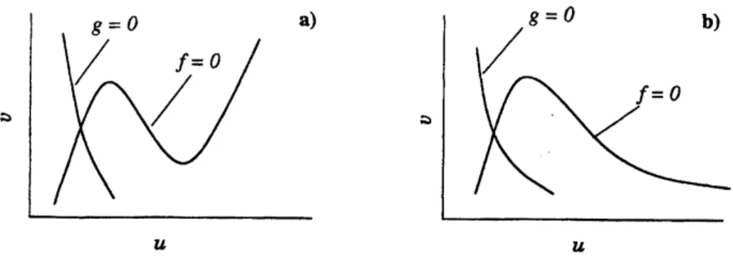
Figure 1: Two major typesofthe nullclnes: $\mathrm{N}$-systems(a) andA-systems (b).

anegativefeedbackbetween$u$and$v$

.

Mathematically,thiscanbe expressed via the$\mathrm{f}\mathrm{o}\mathrm{U}\mathrm{o}\mathrm{w}\mathrm{i}\cdot \mathrm{g}$inequalities

obeyed by the nonlinearities$f$ and$g[26,29]$:

$f_{u}>0$ for

some

$u$,$v$, (1.3)

$g_{v}<0$ for all $u$

,

$v$, (1.4) $f_{v}>0$, $g_{u}<0$

or

$f_{v}<0$, $g_{u}>0$ for all $u,v$

.

(1.3)

The inequality in Eq. (1.3)

means

that small homogeneous increase in $u$ may result in

an

increase in

the production of$u$, the

one

in Eq. (1.4) implies that small homogeneous increasein $v$ will result in

a

decreasein theproduction of$v$, and the

ones

in Eq. (1.5) imply that small homogeneous increase in _$u$

willresult in suchachange in theproductionof$v$that $\mathrm{w}\mathrm{i}\mathrm{U}$resultin

the decrease in theproductionof$u$

.

One

can

distinguish two majorclasses of nonlinearities $f$ and$g$ satisfying Eqs. (1.3) –(1.5). In the

first class, for agiven value of$v$the condition in Eq. (1.3) is satisfiedonly

on

singlebounded interval of

values of$u$

.

In the secondclass, the condition in Eq. (1.3) is satisfied

on a

semi-infinite interval of the

valuesof$u$

.

It isnot difficult to

see

that thisimpliesthat the nullcline ofEq. (1.1) (thatis, the solution of

equation $f(u, v, A)=0$in the$u,v$-plane may be N- or$\mathrm{n}$-shaped, whilein thesecond

case

thisnullcline

may be V-

or

A-shaped (Fig. 1). Therefore, depending

on

the shape of the activator nullcline

one can

classifyreaction-diffusionsystemsof activator-inhibitortypeinto N-orA-systems (thefl- and V-systems

are

equivalent to the former, up to achange ofvariables). This classificationwas introduced by Kerner

and Osipov in [25,26,28, 29]. It is not difficult to verify that the classical Brusselator model [48] is

a

A-system, the Gierer-Meinhardtmodel [14] is

a

$\mathrm{V}$-systems, and the FitzHugh-Nagumo model

$[12,47]$ is

an

$\mathrm{H}$-system. Itturnsout

that the properties ofA-and$\mathrm{V}$-systems arefundamentally differentfrom those

ofN- and Pl-systems [29].

Inthefollowingwewill be considering only$\mathrm{N}$-systems, since thesearethe systems that cangenerate

interfacialpatterns [29,43,44]. Note that$\mathrm{N}$-systems correspondto the

first

case

inEq. (1.5). Furthermore,

we

will restrict ourselves to monostable systems. In other words,

we

will

assume

that the homogeneous state $u=u_{h}$, $v=v_{h}$, satisfying

$f(u_{h},v_{h}, A)=0$, $/(w, v,A)=0$, _(1.6)

is unique for each value of$A$, and that furthermore the point _{$(u_{h}(A),v_{h}(A))$ in} the _$(u,v)$ plane traces continuously the three monotonic branches of the activator nullcline. Physically, this

means

that the controlparameter$A$

measures

the degree ofnonequilibiumin the system.

We will giveanexampleof aderivation ofamodelof the consideredtype inarealistic physical context

inthe next section. Now, however, consider the followingcanonical example [29, 44, 64]:

/$(\mathrm{w},v, A)$ $=$ $u-u^{3}+v$, (1.7)

$g(u, v, A)$ $=$

$A-u-v$

.

(1.8)

Itiseasyto

see

that inthis

case

$f_{u}=1-3u^{2}>0$for $|u|<7^{1}s$ and negative otherwise, $f_{v}=1$,$g_{u}=-1$

,

$g_{v}=-1$,

so

all the above conditions

are

satisfied. Furthermore_{the parameter}$A$hasthe required property, since

$u_{h}=A^{1/3}$, $v_{h}=-A^{1/3}(1-A^{2/3})$

.

_(1.9)

This homogeneous state is stablefor all values of$\alpha$ and$\epsilon$ when $|A|>\nabla\epsilon^{1}\epsilon^{=}$

.

$n_{\mathit{0}}$

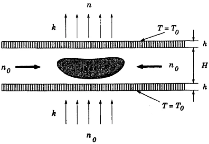
Figure 2: Combustionin acontinuous flow reactor.

2Example:

system with uniformly

generated combustion

ma-terial

Asaprototypicalreaction-diffusionsystemsofactivator-inhibitortype, consideracontinuous flowreactor

withporouswalls inside which

an

exothermic reaction (e.g.,combustion)takes place(Fig. 2). The reactor

is placed between two porous walls ofthickness $h$ andis maintained at the ambient temperature $T_{0}$

on

the outside. Gaseousfuel-0xidizermixture is pumped with rate$k$(with the dimension ofspeed) through

one

of the walls intothe reactor, and the products

are

removed from the other wall with the

same

rate. The reaction releases heat whichis thenabsorbed by the reactor walls.

Ifoneneglects the hydrodynamiceffects, one canwritedown asystemof reaction-diffusion equations

describing the reaction inside the reactor (in three-dimensions) with appropriate boundary conditions

on the reactor walls [65]. The situation may be simplified ifthe distance $H$ between the reactor walls

is small. In this case both the temperature and fuel concentration will vary little between the reactor

walls. Then this system of equations

can

be averaged over the reactor thickness to obtain

an

effective tw0-dimensional reaction-diffusion systemfor theaverage concentration offuel $n$ and temperature$T$ (in energyunits)

across

the reactor:

$\frac{\partial n}{\partial t}$

$=$ $D \Delta n+\frac{k}{H}(n_{0}-n)-\nu ne^{-E_{a}/T}$, (2.1)

$c \rho\frac{\partial T}{\partial t}$

$=$ $\kappa\Delta T$$+ \nu nEe^{-E_{a}/T}-\frac{2\kappa_{wall}}{hH}(T-T_{0})$

.

(2.2)

Here, $D$ is the diffusion coefficient of the fuel, $\kappa$ isthe thermal conductivity of the mixture and $\kappa_{wa}\iota\iota$ is

that of the walls (assumed to be small), $h$ is the wall thickness; $c$ is specific heat and $\rho$ is the density

ofthe mixture. The second term in the right-hand side ofEq. (2.1) is the supply and removal ofthe

fuel withthe incomingfuel concentration $n_{0}$, the last term in the right-handsideof this equationis the

rateatwhich the fuel is consumed, this rate is characterizedbytherate constant $\nu$ (forsimplicity taken

to be temperature-independent), the Arrhenius factor $e^{-E_{\alpha}/T}$, where $E_{a}$ is the activation energy, and

we assumed afirst-0rder reaction. Similarly, the second term in the right-hand side of Eq. (2.2) is the

rate ofheat release by the reaction, with $E$ being the heat released in asingle reaction, and the last

term is the cooling rate. We assumedthat the oxidizer is in

excess

andneglected the dependence of the

transport coefficients

on

temperature. Note that this kind of model

was

introducedphenomenologically

in [24, 27, 29,36].

Let

us

introducethe dimensionless variables $u=T/E_{a}$ and$v=n/n_{0}$ and scaletime andlength with $H/k$ and $(DH/k)^{1/2}$, respectively. Then, Eqs. (2.1) and (2.2) can be reduced to theform of Eqs. (1.1)

$v_{\min}$ $v_{0}$ $v_{\mathrm{m}*\mathrm{x}}$ $v$

Figure3: The activator nullcline (closeup). and (1.2) with

$f=Ave^{-1/u}+u_{0}-u$_, $g=1-v-\gamma ve^{-1/u}$, _(2.3)

$A= \frac{n_{0}\nu hHE}{2\kappa_{wall}E_{a}}$, $\gamma=\frac{\nu H}{k}$, $u_{0}= \frac{T_{0}}{E_{a}}$, (2.4) $\alpha=\frac{c\rho hk}{2\kappa_{wall}}$, $\epsilon$ $=\sqrt{\frac{\kappa hk}{2\kappa_{wall}D}}$

.

(2.5)

Itisnot difficult toverifythat the obtained nonlinearities

are

thoseof

an

$\mathrm{N}$-system. The role of

activator

is playedby the scaled temperature, and the role of inhibitor by the scaled fuel density. This is easyto

understand: the therm0-activatedcharacterofthe reaction results in the positivefeedbackwith respect totemperature, while the consumptionof fuel bythis reaction gives anegativefeedback. Furthermore,

the parameter$A$representsthedegreeofdeviationof the_systemfrom equilibrium, since it is_proportional

to the concentration$n_{0}$ offuel being supplied; the

more

fuelis supplied the further away the systemis

from equilibrium. Then, under aPpropriateconditions this system

can

sustain spatiotemporal patterns.

Physically, the simplest pattern in the form of ahot spot

can

be maintained by the balance of fuel

consumption and supply throughdiffusionfromthe regions away from the spot (Fig. 2).

3Free boundary

problem

A freeboundary problem arises in the analysis of Eqs. (1.1) and (1.2) in the asymptotic limits $\epsilonarrow 0$

$\mathrm{a}\mathrm{n}\mathrm{d}/\mathrm{o}\mathrm{r}\alphaarrow 0$when the nullclne of Eq. (1.1) is$\mathrm{N}$-shaped. Let

us

illustrate this for the

case

when both

$\epsilonarrow 0$and$\alphaarrow 0$whichwewillconcentrate upon in this paper. Clearly, inthislimit the diffusion term in

Eq. (1.1) canbesettozeroonthetimescale$O(1)$

.

Furthermore,for$\alphaarrow 0$and smooth initialconditions

the value of $u$ at each point $x$ will immediately approach $h_{\pm}(v)$, where $h_{+}(v)$ and $h_{-}(v)$

are

the two

stable (inthe

sense

ofthe ODE obtained from Eq. (1.1) with $\epsilon=0$) branchesof the activatornullcline

(see Fig. 3). The choice between these two branches will be dictated by whether the initial condition

for $u$ at each point $x$ lies above

or

below the unstable branch _{$h_{0}(v)$} of the nullcline; those points that

lie below it will end up

on

$h_{-}(v)$, while those above

on

$h_{+}(v)$

.

Thus, thesystems will instantly break

uP into regions $\Omega\pm \mathrm{i}\mathrm{n}$ which

$u$is close to thebranch $h_{\pm}(v)$

,

respectively, separated by the interface $\Gamma$,

possibly disconnected (hence, thecharacterization ofthe stateofthe system

as

adomainpattern). Let

us

emphasizethat

on

thesetimescales the location of$\Gamma$willbe fixedby the initial conditions.

Motion of the interface will

occur on

_{the longer time scale following the interface formation after the}

initialtransient. In order to understandit,

we

need to

zoom

in

on

the interface. Suppose that at time$t_{0}$

we

have$\Gamma$passing through point

$x_{0}$

.

Introducing

$\tau=\frac{t-t_{0}}{\alpha}$

,

$\xi=\frac{x-x_{0}}{\epsilon}$

,

(3.1)

in the limit $\epsilonarrow 0$ and $\alphaarrow 0$ we will get

$u_{\tau}=\Delta\epsilon u+f$(_$u,v$($x_{0}$,to),$A$), (3.2)

where$\Delta_{\xi}$is the Laplacian inthestretchedvariables,and

we

assumed that$v$does notsignificantlyvary

on

the scales of$\tau$ and$\xi$

.

The problem becomes tricky,however,since the initialconditionsfor$u$in Eq. (3.2)

dependent

on

$\alpha$ and $\epsilon$

.

Indeed, thesemustbe approaching $h_{\pm}(v(x_{0}, t_{0}))$

on

therespectivesides of

$\Gamma$and

havenearlyflatlevel sets to be consistentwiththe discussion above. Now, it is knownthat at times$\tau>>1$

flat initial conditions of thistypedevelop into traveling

wave

solutions$u(\xi,\tau)=\overline{u}(\hat{n}\cdot\xi-c\tau)$ moving with

speed$c$inthedirectionof$\hat{n}$ (theunit normal vector to$\Gamma$pointinginthe directionof0)[11]. Therefore,

during interfacialmotionthe profiles of$u$ in theneighborhood of$\Gamma$ should beclose tothe solutionsof

$\overline{u}’-c\overline{u}’+f(\overline{u},v, A)=0$, $\overline{u}(\pm\infty)=h\pm(v)$, (3.3)

in which $v$ is treated

as

aconstant. Small curvature introduces acorrection to the propagation speed,

equal $\mathrm{t}\mathrm{o}-K$, where $K$ is $(n-1)\mathrm{x}$

mean

curvatureofthe interface, positive if$\Gamma$ is

convex

when looked

from $\Omega_{+}$ (see,for example, [10]).

The free boundary problem is obtained from all this via aself-consistency argument. That is,

we

demandthat attime $t$ each point $r$

on

$\Gamma$

move

along thenormal_{$\hat{n}(r,t)$} to$\Gamma$ inthe direction of$\Omega_{-}$ with

the shows mentionedspeed, which isnow afunction ofthe instantaneousvalue of the inhibitor$v(r, t)$ at

point$r$

on

$\Gamma$anditscurvature$K(\mathrm{r})$

.

The distribution of$v$,in turn,satisfiesEq. (1.2) in which$u=h\pm(v)$

in$\Omega\pm$, respectively. Going backtothe original variables,

we

finally obtain

$r_{t}$ $=$ $\alpha^{-1}\epsilon\hat{n}(r)[c(v(r, t), A)-\epsilon K(r)]$, (3.4) $v_{t}$ $=$ $\Delta v+g(h_{\pm}(v), v, A)$, $f(h\pm(v),v,A)=0$

.

(3.3)

Note that this typeof reduction ofasystemofreaction-diffusionequationsto afreeboundary problem

goes back to Fife [9]. For reaction-diffusion systems of activator-inhibitor type in

one

dimension this

reduction

was

used by Nishiura andMimura [51] and by Ohta, Ito, and Tetsuka [54] to study the onset of oscillatory instabilities. Also, in higher dimensions this approach

was

first usedby Ohta, Mimura, and Kobayashiforthe stabilityanalysis of localizedpatterns inaparticular activator-inhibitor model [55].

Before concluding this section, let

us

mention that

an

important class ofreaction-diffusion systems

with theconsiderednonlinearities ischaracterizedbysmall value of$\alpha$and$\epsilonarrow\infty$

.

By asimple rescaling,

these s0-called excitable systems

are

described by Eqs. (1.1) and (1.2), with the diffusion term being

absentin thesecond equation. These systems

are

capableof supporting varioustypes ofwave patterns, includingsolitarywaves,

wave

trains, spiralwaves,andmorecomplexautowave patterns(see,forexample,

[18,35, 63, 64]$)$

.

Free boundary methods have been successfully used for the analysis of anumber of

problemsin these systems. Inparticular, in weaklyexcitablesystems thefree boundaryproblemreduces

to the analogue of asingle Eq. (3.4) (since $v$ is always close to $v_{h}$ in this situation); in this

case a

nice characterization of motion of the interface in the plane

was

introduced by Brazhnik, Davydov,

and Mikhailov $[4, 35]$

.

Using this approach, Brazhnik constructed exact solutions of the free boundary

problem for $\mathrm{V}$-shaped

waves

[3]. Also, Karma worked out the asymptotics of the spiral wave solutions

for$\mathrm{N}$-systems both in theweakly and stronglyexcitable

case

$[19,20]$

.

4Reduced

free

boundary problem

The free boundary problem in Eqs. (3.4) and (3.5) represents asignificant reduction ofcomplexity by

decreasingtheeffective dimensionality of the problem. Nevertheless, it isstill afundamentally nonlinear

problem. In addition to the basic nonlinearity associated with the coupling between the shape of $\Gamma$

and the inhibitor field $v$, which determines the evolution of$\Gamma$, two other

sources

of nonlinearityexist.

The first is the dependence$c(v, A)$ in Eq. (3.4). This dependence is obtained by solving the nonlinear

eigenvalue problemin Eq. (3.3). Phase plane analysis shows that this equation gives auniquevalueof

$c$ for each given $v\mathrm{m}\mathrm{i}\mathrm{n}<v<v_{\max}$ (see, for example, [11]). Furthermore, for smooth nonlnearities the

speed $c$is bounded and changes continuously from anegative value for$v arrow v\min$, since$f(u,v \min, A)\leq 0$

for all values of$u \geq h_{-}(v\min)$ (recall that in $\mathrm{N}$ systems $f_{v}>0$), to apositive value of$c$ for $varrow v_{\max}$,

sincenow $f(u, v_{\max},A)\geq 0$ for all$u\leq h_{+}(v_{\max})$, see also Fig. 3. Moreover, there is auniquevalue of

$v=v0(A)$ _{at which the speed} $c$is

zero.

The value of$v\mathit{0}$ canbe found from the algebraic equation [9] (see

also [21, 22, 29, 37]$)$

$\int_{u-}^{u}+f(u, v_{0}, A)du=0$, (4.1)

where $u_{\pm}=h_{\pm}(v_{0})$

.

Uniquenessof$v_{0}$follows from the monotonic dependence ofthe integral in Eq. (4.1)

on

$v$

.

For example, in the exactly solvable

case

ofthe nonlinearity in Eq. (1.7) the speed $c$ satisfies

implicitly $c- \frac{2}{9}c^{3}=7^{3}2v|$

.

in this case $v_{0}=0$, $u\pm=\pm 1$, $v_{\mathrm{m}\mathrm{i}\mathfrak{n}}=- \frac{2}{3\sqrt{3}}$ and $v_{\max}= \frac{2}{3\sqrt{3}}[38]$

.

The

correspondingfront solution has the form of adomain wall connecting $u_{-}$ with $u_{+}[9, 21,22,29,37]$

.

Thesecond

source

ofnonlinearity mentioned aboveis the functions $h_{\pm}(v)$

.

Note that these functions

are

onlydefinedfor$v\geq v_{\min}$ and$v\leq v_{\max}$, respectively. Therefore, ifduringtheevolution of$\Gamma$the value

of$v$ reachesthese critical values, ajump of the value of$u$from

one

branch ofthe nullclineto the other

must occur. This phenomenon

was

termed local breakd ownby Kerner and Osipov [23,28,29] and inthe

language of the free boundaryproblem amounts to the creation ofnew interface.

The two nonlinear aspectsmentioned above

can

beeliminated if$v(x, t)$ deviateslittle from $v_{0}$ for all $x$. Clearly, this should be the

case

for $v(r, t)$ in astationary pattern,

see

Eq. (3.4). In fact, this is

a

generic situationfor stablestationary patterns in dimensions$n\geq 2[39-44,53]$

.

Introducing

$\tilde{v}=v-v_{0}$, (4.2)

we

can

linearize both thedependence $c(v, A)$ and$h_{\pm}(v)$around$v_{0}$, if $|\tilde{v}|<<1$

.

As aresult, tothe leading

order weobtain $[38,40]$:

c $=b\tilde{v}$, (4.3)

where

$b= \frac{\int_{u-}^{u}+f_{v}(u,v_{0},A)du}{\int_{u-}^{u_{+}}\sqrt{-2U(u,v_{0},A)}du}$ , _{$U(u, v_{0}, A)= \int_{u-}^{u}f(s,v_{0}, A)ds$}

.

(4.4)

Note that for$\mathrm{N}$-systems

we

have$b>0$

.

Similarly, Eq.

(3.5) simplifies to $[38,40]$

$\tilde{v}t$ _{$=$ $\Delta\tilde{v}-(c_{+}\chi_{+}+c_{-}\chi_{-})\tilde{v}+\mathrm{g}(\mathrm{u}_{-}, v_{0}, A)-a\chi_{+}$} (4.5)

where$\chi\pm \mathrm{a}\mathrm{r}\mathrm{e}$ thecharacteristic functions of$\Omega_{\pm}$, and

$a$ $=$ $g(u_{-}, v_{0}, A)-g(u_{+},v_{0}, A)$, (4.6)

$c_{\pm}$ $=$ $-g_{v}(u_{\pm},v_{0}, A)+ \frac{g_{u}(u_{\pm},v_{0},A)f_{v}(u_{\pm},v_{0},A)}{f_{u}(u_{\pm},v_{0},A)}$, (4.7) Observethat by Eqs. (1.3) $-(1.5)$_{, and the fact that} $f_{u}(u_{\pm}, v_{0}, A)<0$ (recall that $u\pm 1\mathrm{i}\mathrm{e}$

on

the stable

branches ofthe nullcline) for $\mathrm{N}$-systems

we

have

$a>0$ and $c_{\pm}>0$

.

For example, in the

case

of the

nonlinearities in Eqs. (1.7) and (1.8) it is not difficultto checkthat $a=2$, $b= \frac{3}{\sqrt{2}}$, $c_{\pm}= \frac{3}{2}$

.

Thus,thereduced free boundaryproblem isobtained fromEq. (3.4)together withEqs. (4.3)and (4.5).

To proceed, weneed to specify the relationship between the parameters$\epsilon$, $\alpha$, and $A$,

as

well

as

thetyPe

ofpattern. Before

we

consider severalparticularcases, let

us

investigate the balance of different terms in

this free boundary problem. The crucial feature of reaction-diffusion systems of activator-inhibitor type

is thatthey

are

capable to support autosolitons –self-sustained inhomogeneous localized patterns [29].

In N-systems in dimensions $n\geq 2$, an autosoliton is asingle radially-symmetric domain $\Omega_{+}$ (or $\Omega_{-}$)

embedded into the whole of$\mathrm{R}^{n}$

.

If _$R$ is the radius of

$\Omega_{+}$ and $T$ is the time scale of its variation,

we

obtainthat different termsin Eqs. (3.4) and (4.5) together with Eq. (4.3) balance each other if

$\frac{R}{T}\sim\frac{\epsilon\overline{v}}{\alpha}\sim\frac{\epsilon^{2}}{\alpha R}$,

$\frac{\overline{v}}{T}\sim\frac{\overline{v}}{R^{2}}\sim 1$

.

(4.8)

where here and below $”\sim$”denotes

an

order of magnitude, and

we

took into account that

$|\tilde{v}|<<1$

.

Note

that this requires that$g(u_{-}, v_{0}, A)$ besmall, which implies that$u_{-}$ and$v_{0}$

are

close to the homogeneous

state $uh$,$v_{h}$

.

Let

us

define the values of$A_{b}^{\pm}$ to be the solutionsof

$g(u_{\pm}(A_{b}^{\pm}),v_{0}(A_{b}^{\pm})$,$A_{b}^{\pm})=0$, (4.9)

where werecalled that $v_{0}$ and $u_{\pm}$

are

in general all functions of$A$

.

We will

assume

that

$A_{b}^{\pm}$ exist and

arealsounique. The values of$A_{b}^{\pm}$ have the meaning ofthecritical values of$A$ at whichthe formation of

localized$\Omega_{\pm}$ patternsis possible [29]. Therefore, by continuity the value of$A$must be close to the value

’

One can seethat the relations in Eq. (4.8) can be satisfied onlyif

$R\sim\epsilon^{1/3}$, $T\sim\alpha\epsilon^{-4/3}$, $\alpha\sim\epsilon^{2}$

.

(4.10)

The consistency of these arguments isverifiedby checkingthat indeed$\tilde{v}\sim R^{2}\sim\epsilon^{2/3}\ll 1$

.

The estimate

in Eq. (4.10), although rather crude, allowsto make anumber of conclusions about the ffee boundary

problem in Eqs. (3.4), (4.3), and (4.5). First, it identifies the precise scaling for the length scale of the

domain patterns. In fact, this scalingwasfirst obtainedfrom the stability considerations ofthe localized

patterns in $\mathrm{N}$-systems in dimensions $n\geq 2[43,44]$, and from theenergetic considerations in the

case

of

extended domain patterns $[39,42]$

.

Second,it gives the scaling for$\alpha$at which the delayinthe response of

the inhibitorbecomessignificant; this scaling has also beenobtainedfrom the stability considerations for

the localizedpattern [43], however,the situation is

more

complicatedforextended patterns (see below).

Also note that the situation is qualitatively different in

one

dimension, in which generically $R\sim 1$ and

$\alpha\sim\epsilon$for the effect ofdelay to appear [24,29,30,50,51,56].

5Applications

We

are now

goingto consider afew applications of the reduced free boundaryproblem which allow to

get major insights into the nonlinear dynamics of interfacial patterns in reaction-diffusion systems of

activator-inhibitortype. For simplicity,

we

willrestrict ourselves totw0-dimensionalpatterns, theresults

remain qualitatively the

same

for all $n>2$

.

Throughout the entire discussionbelow,

we

assume

that

$\epsilon\ll 1$

.

5.1

Self-replication

We first consider the situation in which$A$is close to$A_{b}^{-}$ and the inhibitorisfast,thatis

$\alpha\gg\epsilon^{2}$ (compare

with Eq.(4.10)$)$

.

This

means

thatduringinterfacialmotiontheinhibitor win quicklyequilbrateto reach

a

quasisteady-state,soto theleadingorderthe time derivativein Eq. (4.5)canbe neglected. Furthermore,

if thesize of$\Omega_{+}$ is small,we can neglect the term$c_{+}\chi+\mathrm{i}\mathrm{n}$ this equationaswell. Then Eq. (4.5) can be

easilysolved with the help of Green’s function:

$\tilde{v}(x)=\frac{g(u_{-},v_{0},A)}{c_{-}}-\frac{a}{2\pi}\int_{\Omega}+K_{0}(\sqrt{c_{-}}|x-x’|)dx’$, (5.1) where $K_{0}(x)$ is the modified Bessel function ofthe second kind, and

we

assumedthat $\Omega=\mathrm{R}^{2}$

.

This integral

can

be further reduced to aline integral

over

$\Gamma$

.

In the present context this reduction

was

first performed by Goldstein, Muraki, and Petrich in the

case

of areaction-diffusion system with weak

activator-inhibitor coupling(which

are

necessarilybistable) $[15, 57]$

.

Asimplecalculation shows that if$r$

is apoint

on

$\Gamma$,

we

have

$\tilde{v}(r)=\frac{g(u_{-},v_{0},A)}{c_{-}}+\frac{a}{2\pi\sqrt{c_{-}}}\oint_{\Gamma}(K_{1}(\sqrt{c_{-}}|r-r’|)-\frac{1}{\sqrt{c_{-}}|r-r’|})\frac{(r’-r)\mathrm{x}dr’}{|r’-r|}$, (5.2)

where$K_{1}(x)$ is themodified Bessel function ofthe secondkind, $u\mathrm{x}$”denotes the

cross

product, and$\Gamma$is

assumed to be oriented counterdodcwise with respect to$\Omega_{+}$

.

Now,rescalng length and time according

toEq. (4.10):

$x arrow\frac{\epsilon^{1/3}}{a^{1/3}b^{1/3}}x$

,

$t arrow\frac{\alpha}{\epsilon^{4/3}a^{2/3}b^{2/8}}t$, (5.3)

and expanding the Besselfunction in$\epsilon^{1/3}$, to the leadingorderEq. (3.4) becomes [38]

$r_{t}$ $=$ $\hat{n}(\mathrm{r})$ $(-K(r)$$+\delta$$+ \frac{1}{4\pi}\oint_{\Gamma}(-\Lambda+\ln|r-r’|)(r’-r)\mathrm{x}d\mathrm{r}’)$ , (5.4)

$\delta$$= \frac{b^{2/3}g(u_{-},v_{0},A)}{\epsilon^{2/3}a^{1/3}c_{-}}$, $\Lambda=\frac{1}{3}\ln\epsilon^{-1}+\frac{1}{3}\ln ab-\frac{1}{2}\ln c_{-}+\ln 2-\mathrm{I}+\frac{1}{2}$, (5.5)

and$7\simeq 0.5772$is the Eulerconstant;Aisalarge logarithm. Note that related free boundary formulation

was

discussed by Nishiura and Onishi [52].

To understand the significance of different termsin Eq. (5.4), let

us

consider

an

ideallyround domain

$\Omega_{+}$ first. Then, Eq. (5.4) reduces toasingle ODEfor the domainradius_$\rho[41]$

$\frac{d\rho}{dt}=-\frac{1}{\rho}+\delta+\frac{1}{4}\rho^{2}(-2\Lambda+2\ln\rho+1)$

.

(5.6)

This formula is vald when $\rho$ is not very large, when Ais the dominant term in the right-hand side of

Eq. (5.6). The analysis of this equationthen shows that if the value of$\delta$ is negative in this rangeof

$\rho$

all radially-symmetric domains will shrink to zero in finite time. On the other hand, when $\delta$ becomes

sufficiently largepositive, two equilibria with radii$\rho_{u}<\rho_{0}$ appear, with$\rho_{u}$ being unstable and

Astable

(see also [42]). Furthermore, the radius $\rho 0$ is uniquely determined by

$\delta$ and is $O(1)$ for

$\delta=O(\Lambda)$

.

Note that this is precisely the solution inthe form ofan autosoliton.

Afundamental featureof reaction-diffusion systems ofactivator-inhibitor tyPe in dimensions $n\geq 2$

is thatpatterns

can

undergo morphological instabilities resulting in shape changes [15,29,43-45,55, 58].

Thiscan readilybe seen, if

one

perturbsEq. (5.4)around aradially stable disk-shaped domain of radius

$\rho 0$

.

Introducingpolarcoordinates $(\rho, \varphi)$ for $\Gamma$and substituting_{$\rho(\varphi, t)=\rho_{0}+\rho_{m}e^{tm\varphi-\gamma_{m}t}$}

intoEq. (5.4),

we

thentake alimit of$\rho_{m}arrow 0$toobtain [41-43]

$\gamma_{m}=\frac{m^{2}-1}{\rho_{0}^{2}}-\frac{\rho_{0}}{2}(1-\frac{1}{m})$ , (5.7)

whichis valid for $m>0$

.

From this equationfollows that the radially-symmetric patternundergoes the distortion instability corresponding to $m=2$when $\rho_{0}>\rho_{\mathrm{c}2}=(12)^{1/3}$

.

Qualitatively,

one

can

understand this morphological instability

as

follows. When $\rho\sim 1$,both $\delta$ and

Ain Eq. (5.4)

are

large. Then, since Amultiplies the integral which gives the

area

of$\Omega_{+}$, the effect of

these two terms is basicallyto preserve the pattern’s overall

area.

Incontrast, morphological instabilities preserve the

area

and

are

therefore driven by the $\ln|\mathrm{r}$ $-r’|$ term in Eq. (5.4). Observethat this term

can

be positive if $|r-r’|$ is large and negative when $|r-r’|$ is small. Therefore, its effect will be to

pull apart distant piecesofthe interface. If thesize ofthepatternis large, thenthestabilizing effect of

curvature would not be able to compensatethis tendency, and apattern with complexmorphology will

develop [38,43,44].

The next question here is whether the pattern growing as aresult of this instability will preserve

its topology, namely, whether it will remain connected during the

course

of its evolution. Numerical simulations of reaction-diffusionsystemswith weak activator-inhibitor coupling[16],

as

well

as

simulations

ofthe free boundary problem for these systems [8,15,57] showed that aconnected labyrinthine pattern

formed asaresult of the morphological instability of the disk-shaped domain.

To test this question in the systems under consideration,

we

performed anumerical solution of

Eq. (5.4). The interface

was

discretized

as

apiecewise-linear curve,integration in space

was

done using

midpointrule,curvatureatagivenpoint

was

obtained bydrawing acircle through that pointanditstwo neighbors to obtain anapproximationfor the curvature radius. The number of discretization points

was

controledadaptively tomaintainthedistancebetween the neighboringpointswithinafactor of two. In

ournumerical method,wealso allowed$\Gamma$to reconnect whentheinterfacescamesufficiently close together.

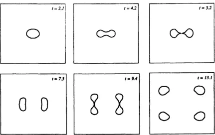
The result ofatypicalsimulationis showninFig. 4. The initial condition is taken

as

aslightlyperturbed

disk-shaped domain ofradius$\rho_{0}>\beta \mathrm{e}2$

.

One

can see

that the domainundergoing instability pinches off

and divides, the daughter domains keep undergoing divisions. Thus, in $\mathrm{N}$-systems with fast inhibitor

self-replication

can

beobservedas aresult of the morphological instability. This is alsoconfirmedinthe

numericalsimulations of the original reaction-diffusion equations with sufficiently small$\epsilon[41,42]$

.

Let

us

point out that the numerical solution of thefreeboundary problem could

run

only until acertain time,

after which the domains started to blow up,

so

only afew acts ofself-replicationcouldbeobserved. We attribute this tothe fact that the replicatingdomains go

so

far apartthat theexpansion used to obtain

t–2.l t–4.2 t–5.2

$\mathrm{O}$ $\infty$ $\propto\triangleleft$

$t=7.\mathit{3}$ $t\overline{-}\mathit{9}.4$ $t\overline{-}J\mathit{3}.\mathit{1}$

$0$ $0$ $\int$ $\int$

O

0

O

$O$

Figure 4: Self-replication ofaspot. Result of the numerical solution ofEq. (5.4). The box is 50$\mathrm{x}50$

.

Other parameters

are:

$\mathrm{A}=4$, $\delta=18.3$, based

on

the model in Eq. (1.7)

an

(1.8) with $\epsilon=10^{-4}$,

$A-A_{b}^{-}=0.0455$

.

Eq. (5.4) from Eq. (5.2) breaks down. When the domains become separatedby distances of order 1(in

the original variables),

one

needs to keep the full Bessel function (which decays exponentially at large

distances) inthe integralin Eq. (5.4). Note that both the phenomenon of self-replication and formation

oflabyrinthinepatterns

were

observedexperimentally in $[31, 32]$

.

5.2

Breathing spot

We

now

turnto the studyof theeffect of the delayintheinhibitorresponseto the motion of the interface.

To do thatconsiderthefollowingsimple setup. Let $\Omega$beadiskofdiameter$L\ll 1$ (but,ofcourse, $L\gg\epsilon$)

and consider aradially-symmetricpattern$\Omega_{+}$ with radius$\mathrm{p}(\mathrm{t})$in$\Omega$

.

Since$\Omega$is small, thespatial variation

of$v$ willbe small

across

0. Therefore, for astationary pattern

we

will

once

again have $|\tilde{v}|<<1$,

so

the

reduced freeboundary problem ofSec. 4should work.

Equation(3.4) inthe considered casebecomes (we arebadc to the unsealedvariables)

$\frac{d\rho}{dt}=-\frac{\epsilon^{2}}{\alpha\rho}+\frac{\epsilon b\overline{v}(\rho,t)}{\alpha}$

.

(5.8)

Toproceed, let

us

break up $\tilde{v}$

as

follows

$\tilde{v}=\overline{v}+\hat{v}$, (5.9)

where $\overline{v}$ is the value of$\tilde{v}$ averaged

over

$\Omega$

.

It turns out that for $\alpha\gg\epsilon^{2}$ the dynamics of$\overline{v}$ and $\tilde{v}$

are

qualitativelydifferent. AveragingEq. (4.5)

over

$x$, weobtain

$\frac{d\overline{v}}{dt}=-(\frac{(L^{2}-4\rho^{2})c_{-}}{L^{2}}+\frac{4\rho^{2}c_{+}}{L^{2}})\overline{v}-\frac{4a(\rho^{2}-\rho_{0}^{2})}{L^{2}}$, (5.10)

where

$\rho_{0}=\frac{L^{2}g(u_{-},v_{0},A)}{4a}$

.

(5.11)

In writing Eq. (5.10),

we

neglected the termcomingfrom$\hat{v}$,which is going tobe smallcompared to the

lastterm inthe right-handside ofthis equationintheconsideredregime (see below).

Toclosethis systemofequations,

we

needtofind$\mathrm{v}(\mathrm{p}, t)$

.

The equationfor$\hat{v}$is obtainedby subtracting

Eq. (5.10)from Eq. (4.5). If

we

also

assume

that$\alpha\gg\epsilon^{2}$,bytheargument similar to the

one

in Eq.(4.10)

we

will

see

that the time derivativeof$\hat{v}$ is small and

can

be dropped from this equation. Similarly, the

value of $\hat{v}$ should

come

out to be oforder$L^{2}$ and therefore will be small compared to the last term in

Eq. (4.5). With allthese reductions,to the leading order the equation for$\hat{v}$ becomes

$\frac{d^{2}\hat{v}}{dr^{2}}+\frac{1}{\mathrm{r}}\frac{d\hat{v}}{dr}-a(\chi_{+}-\langle\chi_{+}\rangle)=0$, (_{$\hat{v}\rangle=0,$} (5.12)

where $r$ isthe radial coordinate and $\langle.\rangle$ denotesspatialaverage. This equation

can

be trivially solved to

obtain

$\hat{v}(\rho)=a(\frac{3\rho^{2}}{8}-\frac{3\rho^{4}}{2L^{2}}+\frac{\rho^{2}}{2}\ln\frac{2\rho}{L})$

.

(5.13)

Let

us

introducethefollowing quantities

$\overline{\rho}=\frac{\rho}{L}$,

$\omega_{0}=\sqrt{\frac{4\epsilon ab}{\alpha L}}$,

$\tau=\frac{\alpha}{\epsilon abL}$, $\overline{\epsilon}=\frac{\epsilon}{abL^{3}}$

.

(5.14)

Assumingthat $\omega_{0}\gg 1$, while$\tau\sim 1$, we canfurther reduce Eqs. (5.8), (5.10), and (5.13) by eliminating

$\overline{v}$to [40]

$\frac{d^{2}\overline{\rho}}{dt^{2}}+\beta(\overline{\rho})\frac{d\overline{\rho}}{dt}+\omega_{0}^{2}(\overline{\rho}^{2}-\overline{\rho}_{0}^{2})=0$, (5.15)

where

$\beta(\overline{\rho})=c_{-}+4(c_{+}-c_{-})\overline{\rho}^{2}-\tau^{-1}(\frac{\overline{\epsilon}}{p}+\frac{5\overline{\rho}}{4}-6\rho^{4}+\overline{\rho}\ln 2\overline{\rho})$

.

(5.16)

We

now

demand that $\tilde{\epsilon}$and

$\overline{\rho}0$

are

$O(1)$ quantities, which implies that $L\sim\epsilon^{1/3}$, $\alpha\sim\epsilon^{4/3}$

.

(5.17)

Equation (5.16) then describes

an

equation for aweakly damped nonlinear oscillator with nonlinear friction coefficient $\beta(\overline{\rho})$

.

Acompletestudy of this dynamical system is possible (foradetailed analysis,

see

[40]$)$

.

Importantly,inawiderangeofpo (implyingarangeof valuesof$A$between$A_{b}^{-}$and$A_{b}^{+}$) aHopf

bifurcationof thestationary solutionwith$\overline{\rho}=\mathrm{p}\mathrm{o}$ is realized at_{$\tau=\tau_{c}$}, where to the leading order [40]

$\tau_{c}=\frac{4\overline{\epsilon}+5\overline{\rho}_{0}^{3}-24\overline{\rho}_{0}^{5}+4\overline{\rho}_{0}^{3}1\mathrm{n}2\overline{\rho}_{0}}{4\overline{\rho}_{0}^{2}(c_{-}+4(c_{+}-c_{-})\overline{\rho}_{0}^{2})}$, (5.18)

which is obtained by simply equating $\beta(\overline{\rho}_{0})$ to

zero

(recall that $\omega_{0}\sim\epsilon^{-1/3}\gg 1$). We emphasize that

these results

are

completely independentofthe original nonlinearities$f$ and$g$

.

Let

us

also point outthat

this behavior

was

experimentally observed in [17].

5.3

Phase

waves

Lastly,

we

will discussthe problem of describing the interactionofdifferent domains in amultidomain

pattern. Thisisafundamentalproblem in the theory ofreaction-diffusionequationsofactivator-inhibitor

tyPe, sincetypically the patterns that form in these systems

are

extended [41,42,44]. Themain obstacle

in doing this is the fact thatgenerally the patternsforming under these conditions

are

highlydisordered

$[41,42]$

.

Another_{problem isthatdifferent domains interact witheachotheron different length scales: the}

localarrangementof domainsinastable stationarypatternisdue totheshort-rangeinteraction between nearest neighbors, while the long-range interactions at distances \sim 1are responsible for the screening effects (see,for example, Eqs. (3.4) and (5.2)).

This problem

can

be simplified if

one

looks at perturbations (not necessarily small) of stationary

periodic patterns. In the followingwe will considerapattern in theform of(nearly-) circular domains

arranged in ahexagonal lattice ofperiod $\mathcal{L}_{\mathrm{p}}$

as an

example. Unless $A$ is close to $A_{b}^{\pm}$, these patterns

are

stable only when $\mathcal{L}_{p}\sim\epsilon^{1/3}[39,41,42]$

.

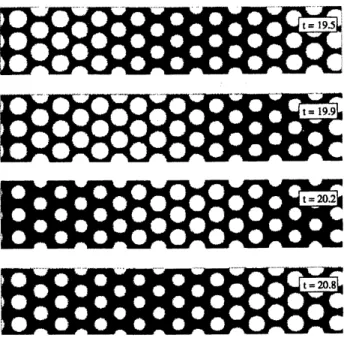
Numerical simulations show that for smaU enough$\alpha$ these

patterns

can

support phase

waves

of oscillations ofthe domain radii (Fig. 5). It is observed that these

Figure 5: Propagationof the

wave

ofcoUectiveoscillationsof the domain radii obtainedfrom numerical

solutionof Eqs. (1.1)and(1.2) withthe nonlinearities givenbyEq.(1.7)and(1.8) and$\epsilon=0.05$,$\alpha=0.02$,

and$A=-0.4$

.

The domainis 20$\mathrm{x}4$

.

The boundaryconditions

are

periodic.

waves

represent slow modulations in space of the periodic breathing motion of individual domains [40].

Note that thesepatterns

are

also realizedin experiments [7].

Onceagain,sincein aperiodic patternof small period the deviation of$v$from$v_{0}$issmall,thereduced

free boundaryproblem ofSec. 4can be applied. Moreover,for not very large domain radii comparedto

$\mathcal{L}_{p}/2$ (in practice, for virtually all radii) the deviations of the domain shape from that ofan ideal disk

can be neglected. Then, to obtain effective equations that describe the slowly varying modulations of the domainradii,

we

introduce thefunction$\mathrm{p}(\mathrm{x}, t)$, whichis thecoarse-grained (smoothed) version ofthe

radiusof

an

individual domain in agiven hexagonal cell. We then separate$\tilde{v}$

as

in Eq. (5.9),where

now

$\overline{v}$ isdefined

as

the

coarse

grainedversion of$\overline{v}$, that is, wetake $\overline{v}$to be the averageof

$\overline{v}$

over an area

of

the size whichismuch greaterthan $\mathcal{L}_{p}$but smallerthan thelength scale ofvariationof$\rho$

.

To the leading

order the equation for $\overline{v}$,

now

also slowly varying in space, becomes

$\frac{\partial\overline{v}}{\partial t}=\Delta\overline{v}-(\frac{(L^{2}-4\rho^{2})c_{-}}{L^{2}}+\frac{4\rho^{2}c+}{L^{2}})\overline{v}-\frac{4a(\rho^{2}-\rho_{0}^{2})}{L^{2}}$,

(5.19).

where$\rho_{0}$ is

as

in Eq. (5.11) and

$L=3^{1/4}2^{1/2}\pi^{-1/2}\mathcal{L}_{\mathrm{p}}$

,

(5.20)

so

that$\pi L^{2}/4$isequaltothe

area

of asingle hexagonal cell. Now,since$\hat{v}$shouldbe small, slowvariations

of$\hat{v}$between different cells$\mathrm{w}\mathrm{i}\mathrm{U}$be higher-0rdercorrectionand

can

beneglected. Therefore,tothe leading

order

we can

solve the problemfor $\hat{v}$in eachhexagonal cell with

no

fluxboundary conditions. Assuming

that $\alpha\gg\epsilon^{2}$ and following the argument of the section above, we obtainthefollowing problem for$\hat{v}$ in

the hexagonalcell$\Omega_{0}$ for each$\rho$:

$\Delta\hat{v}-a(\chi_{+}-(\chi_{+}))=0$, $\langle\hat{v})=0$, $\frac{\partial\hat{v}}{\partial n}|_{\partial\Omega_{0}}=0$, (5.21)

where

now

$($

.

$)$ denotesaveraging

over

$\Omega_{0}$

.

To finally close this system of equations,

we

use

the

average

value of$\hat{v}$

over

the domain’sinterfacein Eq. (5.8):

$\frac{\partial\rho}{\partial t}=-\frac{\epsilon^{2}}{\alpha\rho}+\frac{\epsilon b}{\alpha}(\overline{v}+\frac{1}{2\pi}\int_{0}^{2\pi}\hat{v}(\rho, \varphi)d\varphi)$, (5.22)

wherethe variationsof$\overline{v}$

across

Q

$0$wereneglected and$\hat{v}$on$\Gamma$

was

writtenin terms of the polarcoordinates

$(\rho, \varphi)$ of the interface. Note that it should also bepossibleto obtain theseequationsusing homogenization

techniques. Also note that the deviations from the ideal disk $\mathrm{s}\mathrm{h}\mathrm{a}\mathrm{p}\mathrm{e}\infty$ for each domain

can

be taken into

accountbywritingthe positionoftheinterface

as

$r( \varphi, t)=\rho(t)+\sum_{m=1}\rho_{6m}(t)\cos(6m\varphi)$ in polarcoordinates

and modifying Eq. (5.22) accordingly, together with obtaining equations for each$\rho 6m$

.

The main difficulty in analyzing the equations above must be the solution of Eq. (5.21), which has

to be done in the hexagonal geometry. This problem, however,

can

be handled approximately by the Wigner-Seitz method fromsolidstatephysics (see,forexample,[66]). Namely, instead of solving Eq(5.21) in $\Omega_{0}$, we will solve it

on

adisk ofthe

same area.

This immediately

allows

us

to

use

the results of the

previous section. Once again, introducing the constants from Eq. (5.14) and following the same steps,

we now

arrive at the following effective PDE for$\overline{\rho}(x, t)[40]^{1}$

$\frac{\partial^{2}\overline{\rho}}{\partial t^{2}}+\omega_{0}^{2}(\overline{\rho}^{2}-\overline{\rho}_{0}^{2})=-(\beta(\overline{\rho})-\Delta)\frac{\partial\overline{\rho}}{\partial t}$ ,

(5.23)

where$\beta(\rho)$ is still given by Eq. (5.16). Note that the spatially-independent solutions of this equation

(which correspond to in-phase oscillations of all domains)

are

equivalent to the oscillations ofasingle

domain consideredintheprevioussection. Therefore, this

means

that hexagonalpatternsalso undergo

a

Hopfbifurcationleading to the onset ofsynchronous breathing motion [40]. One

can

further investigate

the dynamic coupling between different domains. Onestrikingobservationhere is that while locally the

domain oscillationssynchronize, globally they

can

exhibit chaotic behavior[40]. Let

us

also point out that similartreatmentof thistyPeofpatternsispossible_foravarietyofgeometries,including

one

dimension,

wherearather complete study of the pattern’sdynamics is possible [40].

6Conclusion

To summarize,

we

have presented

an

overview of recent results

on

the applications of free boundary

problemto reaction-diffusion equations of activator-inhibitor type. This overview was concentrated on

the

case

of long-ranged and slow inhibitor ($\epsilon\ll 1$ and $\epsilon^{2}\ll\alpha\ll 1$). The techniques we used for obtaining the free boundary reduction of the original reaction-diffusionequations

were

based

on

formal

asymptotics and heuristic arguments. Let us point out that most ofthe results obtained in Sec. 5can

besystematically derived via formal asymptoticexpansions of the original reaction-diffusion problem by assuming the aPPropriate scaling relationships between $\epsilon$, $\alpha$

,

and $A$

,

in the limit $\epsilonarrow 0$

.

However,

we

choseto

use amore

intuitiveapproach,since itprovidesinsights into theorigins of these scalingrelations.

We also chose topresentthe

cases

whichlead to interesting phenomenology; otherregimes

can

be studied using similar methods.

To the best of

our

knowledge,rigorous workonthe problemsdiscussed above is quite recent. We first

wouldlike to mentionthe work ofSoraviaand Souganidis who obtained free boundaryreductions for

a

subsetofreaction-diffusion systems of activator-inhibitor type in $\mathbb{R}^{n}$ that

are

valid globallyin time [61].

See also this work for the list of references on existence of solutions to the interfacial problem. More

recently, Bonami, Hilhorst, and Logak analyzed adifferent scaling regime foraparticularmodel $[2, 33]$

.

Their free boundary problem is essentially abounded $\Omega$ version of the problem considered in Sec. 5.1

(except _{for the Dirichlet boundary conditions for} $\tilde{v}$). Adifferent scaling regime

was

investigated by

Sakamoto, with theresults alongthe lines of the discussion at the beginningofSec. 3[60].

Let

us

also point out that in the

case

of fast inhibitor the reduced free boundary problempossesses

an energy functional $[41,42]$

.

This allows to make anumber of_{further conclusions about the dynamics}

of the interfacesand,_{in particular, about the stable stationary patterns, which}

_are

_now

_{local minimizers}

of the_{energy. For acertain scaling, these local minimizers}

_were

_studied by Ren and Wei in the context

ofT-convergence [59]. Also, Choksiobtained precise scalingfor the global energy minimizers [5]. Let

us

point out that these authors essentially consider bounded domains whose size shrinks to

zero

in the

limit $\epsilonarrow 0$

.

This isdifferent from thesituationof$\Omega$ $=\mathrm{R}^{n}$ consideredin

Sec.

5,where twolength scales:

one

of single domain size, $O(\epsilon^{1/3})$, and the other of screening effects, _$O(1)$, exist (naturally,

the third

lThis equation improves slightly the result of [40], where $L$waschosen tobesimply equalto$\mathcal{L}_{p}$inreducing Eq. (5.21)

tothe radialproblem.

lengthscale $O(\epsilon)$ which correspondsto the interfacialthickness, present in the fullsystem of PDEs, does

not enter thefree boundary problem). This mustleadto homogenization-typeproblems andiscurrently

open. In particular, one problem of interest here is the dynamics of patterns with slowly modulated

morphologies.

The

case

of slow inhibitor obeyingthe scalingfromEq. (5.17) andsimilar

cases

has not been analyzed

rigorously yet. Here the

cases

ofbreathing patterns and perturbations ofperiodic patternsconsidered in

Sees. 5.2and5.3seempromising. Moregenerally, afundamental problemin thiscontextisto understand

similar phenomena ofcollective oscillations for disordered domain patterns. In this

case

it is not

even

clear what the starting point for the analysis ofsuch patterns oflargenumbers ofinteracting domains

should be. Onestep inthatdirectionwasmadein [40],where ashadow limit of thereducedfreeboundary

problemwith the initialconditionsin theform of apolydisperse mixtureof radialdropletswasconsidered;

the dynamics of the pattern

on

acertain timescale could thenbe analyzed via astatisticaldescription

involvingthedistribution of thedroplets’ radii.

Theauthor wouldlike toacknowledgevaluablediscussions with V. V. OsipovandS. Y. Shvartsman.

References

[1] E.Ben-Jacob,I. Cohen,andH.Levine.Cooperative self-0rganization in microorganisms. Adv. Phys.,

49:395-554, 2000.

[2] A. Bonami, D. Hilhorst, and E. Logak. Modified motion by

mean

curvature: local existence and

uniqueness andqualitativeproperties.

_Differential

Integral Equations, 13:1371-1392,2000.

[3] P. K. Brazhnik. Exact solutions for the kinematic model of autowavesin two dimensional excitable

media. Physica D, 94:205-220,1996.

[4] P. K. Brazhnik, V. A. Davydov, and A. S. Mikhailov. Akinematic approach to the description of

autowave processes in active media. Theoret. and Math. Phys., 74:300-306, 1988.

[5] R. Choksi. Scaling laws in microphase separationof diblockcopolymers. J. Nonlinear Sci., $11:22\succ$

236,2001.

[6] M. Cross and P. C. Hohenberg. Pattern formation outside ofequilibrium. Rev. Mod. Phys.,

65:851-1112, 1993.

[7] P. De Kepper, J.-J. Perraud, B. Rudovics, and E. Dulos. Experimental study ofstationary Turing

patterns and their interaction with traveling

waves

in achemical system. Int. J.

_Bifurc.

Chaos,

4:1215-1231, 1996.

[8] C. Elphick, A. Hagberg, and E. Meron. Dynamic front transitions and spiral-vortex nucleation.

Phys. Rev. E., 51:3052-3058,1995.

[9] P. C. Fife. Pattern formationin reacting and diffusing systems. J. Chem. Phys., 64:554-564,1996.

[10] P. C. Fife. Dynamics

_of

Internal Layers and

_{Diffusive Interfaces.}

Society forIndustrial and Applied Mathematics, Philadelphia, 1988.

[11] P. C.Fife and J. B.McLeod. The approach of solutions of nonlinear diffusion equations to traveling front solutions. Arch. Rat. Mech. Anal., 65:335-361, 1996.

[12] P.G.FitzHugh. Mathematical models ofexcitation and propagation in

nerve.

Biophys. J., 1:445-466,

1961.

[13] M. Freeman and J. B. Gurdon. Regulatory principles in developmental signalng. Annu. Rev. Cell

Dev. Biol, 18:515-539, 2002.

[14] A. GiererandH. Meinhardt. Atheoryof biological pattern formation. Kybernetik, 12:30-39,1996.

[15] R. E. Goldstein, D.J.Muraki,andD. M.Petrich. Interface proliferation andthe growthof labyrinths

inareaction-diffusion system. Phys. Rev. E, 53:3933-3957,

1996.

[16] A. Hagberg and E. Meron. Prom labyrinthine patterns to spiral turbulence. Phys. Rev. Lett,

72:2494-2497, 1994.

[17] D.Haim,_{G. Li,}Q. Ouyang, W. D.McCormick,H. L.Swinney,A. Hagberg,andE. Meron. Breathing

spots in areaction-diffusionsystem. Phys. Rev. Lett, 77:190-193, 1996.

[18] R. KapralandK. Showalter, editors. Chemical

waves

and patterns. Kluwer, Dordrecht, _1995.

[19] A. Karma. Universal limit of spiral

wave

propagationinexcitable media. Phys. Rev. Lett,

66:2274-2277 1991.

[20] A. Karma. Scaling regime of spiral

wave

propagation in single-diffusive media. Phys. Rev. Lett,

$68:397\triangleleft 00$,1994.

[21] B. S. Kerner and V. V. Osipov. Nonlinear theory of stationary stratain dissipative systems. Sov.

Phys. –JETP, 47:874-885, 1978.

[22] B. S. KernerandV. V. Osipov. Stochastically inhomogeneousstructuresin nonequilibrium systems.

Sov. Phys. –JETP, 52:1122-1132,1986.

[23] B. S. Kerner and V. V. Osipov. Dynamic rearrangement of dissipative structures.

Sov.

Phys.

-Doklady, $27:484\triangleleft 86$,1986.

[24] B. S. Kerner and V. V. Osipov. Pulsating “heterophase” regions in nonequilibrium systems. Sov.

Phys. –JETP, 56:1275-1282,1986.

[25] B. S. Kerner and V. V. Osipov. Autosolitons in activesystems with diffusion. In W. Ebeling and

H. Ulbricht, editors, Self-Organization bynonlinear irreversible processes. Springer, NewYork, 1986.

[26] B. S. Kernerand V.V. Osipov. Autosolitons. Sov. Phys. –Uspekhi, 32:101-138, 1989.

[27] B. S. Kernerand V. V. Osipov. Thermal diffusion autosolitonsinsemiconductor andgasplasmas. In

A. V. Gaponov-Grekhov,M.I. Rabinovich, and J. Engelbrecht, editors, NonlinearWaves: Dynamics

andEvolution. Springer-Verlag, Berlin, 1989.

[28] B. S. KernerandV. V. Osipov. Self-0rganizationinactivedistributedmedia. Sov. Phys. –Uspekhi,

33:679-719,

1990.

[29] B. S. KernerandV. V. Osipov. Autosolitons: aNew Approach to Problems

_of

Self-Organizationand

$\mathrm{f}\mathrm{f}\mathrm{l}\iota$fbulenoe. Kluwer, Dordrecht, 1994.

[30] E. M. Kuznetsova and V. V. Osipov. Properties of autowaves including transitions between the travelingandstatic solitary states. Phys. Rev. E, 51:148-157, 1995.

[31] K.LeeandH.Swinney. Lamellarstructuresandself-replicatingspotsin areaction-diffusionsystem.

Phys. Rev. E, 51:1899-1915,1995.

[32] K. J. Lee, W. D. McCormick, Q. Ouyang, and H. L. Swinney. Experimental observation of self-replicating chemical spots in areaction-diffusionsystem. Nature, 369:215, 1994.

[33] E. Logak. Singularlimitof reaction-diffusionsystems andmodified motionby

mean

curvature. Proc.

Roy. Soc. Edinburgh Sect A, _{132:951-973, 2002.}

[34] A. G. Merzhanov and E. N. Rumanov. Physics ofreaction

waves.

Rev. Mod. Phys., 71:1173-1210,

1999.

[35] A. S. Mikhailov. Foundations

_of

Synergetics. Springer-Verlag,Berlin,

1990.

[36] M. Mimura, M. Nagayama, and K. Sakamoto. Pattern dynamics in

an

exothermic reaction. Physica

D, 84:58-71, 1995.

[37] M. Mimura, M. Tabata, and Y. Hosono. Multiple solutions of two point boundary value problems of

neumann

typewith asmall parameter. SIAM J. Math. Anal, 11:613-631, _1986.

[38] C. B. Muratov. Self-replication and splitting ofdomain patterns in reaction-diffusionsystems with

the fastinhibitor. Phys. Rev. E, 54:3369-3376, 1996.

[39] C. B. Muratov. Instabilities and disorder ofthe domain patterns in the systems with competing

interactions. Phys. Rev. Lett, 78:3149-3152,1997.

[40] C. B. Muratov. Synchronization, chaos, and the breakdownofthe collective domain oscillations in

reaction-diffusion systems. Phys. Rev. E, 55:1463-1477, 1997.

[41] C. B. Muratov. Theory

of

domain patterms in systems with long-range interactions

_of

Coulombic

type. Ph. D. Thesis, BostonUniversity, 1998.

[42] C. B. Muratov. Theory of domainpatternsin systems with long-rangeinteractionsofcoulombtype.

Phys. Rev. E, 66:066108,2002.

[43] C. B. Muratov andV. V. Osipov. Generaltheoryofinstabilities for patternwith

_sharP

interfaces in

reaction-diffusionsystems. Phys. Rev. E, 53:3101-3116,1996.

[44] C. B. Muratov and V. V. Osipov. Scenarios of domain pattern formation in

areaction-diffusion

system. Phys. Rev. E, 54:4860-4879, 1996.

[45] C. B. Muratov and V. V. Osipov. Stability ofstatic spike autosolitons in the Gray-Scott model.

SIAMJ. Appl. Math., 62:1463-1487,2002.

[46] J. D. Murray. Mathematical Biology. Springer-Verlag,Berlin, 1989.

[47] J. Nagumo, S. Arimoto,andS. Yoshizawa. An active pulsetransmissionline simulating

nerve axon.

Proc. IEEE, 50:2061-2070, 1989.

[48] G.Nicolis and I. Prigogine. Self-Organization in Non-Equilibrium Systems. Wiley Interscience,New

York, 1977.

[49] F. J. Niedernostheide, editor. Nonlinear dynamics andpattern

_formation

in semiconductors and devices. Springer, Berlin, 1994.

[50] Y. Nishiuraand H. Fujii. Stability ofsingularly perturbedsolutionsto systemsofreaction-diffusion

equations. SIAMJ. Math. Anal, 18:1726-1770,1997.

[51] Y. Nishiura and M. Mimura. Layeroscillations inreaction-diffusionsystems. SIAMJ. Appl. Math.,

49:481-514, 1989.

[52] Y. Nishiura and I. Ohnishi. Some mathematical aspects of the micr0-phase separation in diblock

copolymers. PhysicaD, 84:31-39, 1995.

[53] Y. Nishiura and H.Suzuki. Nonexistence ofhigher-dimensionalTuringpatterns inthe singular limit.

SIAMJ. Appl. Math., 29:1087-1105,1998.

[54] T. Ohta, A. Ito, and A. Tetsuka. Self-0rganization in

an

excitable

reaction-diffusion

system:

syn-chronization of oscillating domainsin

one

dimension. Phys. Rev. A, 42:3225-3232,1996.

[55] T. Ohta, M. Mimura, andR. Kobayashi. Higher-dimensional localizedpatterns inexcitable media.

Physica D, 34:115-144, 1989.

[56] V. V. Osipov. Criteria ofspontaneousinterconversionsof travelingand staticarbitrarydimensional

dissipative structures. Physica D, 93:143-156, 1996.

[57] D. M. Petrich and R. E. Goldstein. Nonlocal contour dynamics model for chemical front motion.

Phys. Rev. Lett., 72:1120-1123, 1994.

[58] L. M. Pismen. Turing patterns and solitary structures under global

control.

J. Chem. Phys.,

101:3135-3146,

1994.

[59] X. F. Ren and J. C. Wei. On the multiplicity of solutions oftwo nonlocal variational problems.

SIAMJ. Math. Anal., 31:909-924, 2000.

[60] K. Sakamoto. Spatial homogenization andinternal layers in areaction-diffusion system. Hiroshima

Math. J.,30:377-402, 2000.

[61] P. Soraviaand P. E. Souganidis. Phase field theory for FitzHugh-Nagumo-type systems. SIAM J.

Math. Anal., 27:1341-1359,1952.

[62] A. M. Turing. The chemical basis ofmorphogenesis. Phil. Trans. R. Soc. London B, 237:37-72,

1952.

[63] J.J. Tyson and J. P. Keener. Singular perturbation theory of travelng

waves

inexcitable media (a

review). Physica D, 32:327-361,_1987.

[64] V. A. Vasiliev, Yu. M. Romanovskii, D. S. Chernavskii, and V.G. Yakhno.

Autowave

Processes in

Kinetic Systems. VEB DeutscherVerlagder Wissenschaften, Berlin, 1987.

[65] Ya. B. Zeldovich, G. I. Barenblatt, V. B. Librovich, and G. M. Makhviladze. The Mathematical

Theory

_of

Combustion andExplosions. ConsultantsBureau, New York, 1985.

[66] J. M. Ziman. Principles

_of

the Theory

_of

Solids. Cambridge University Press, Cambridge, 1972