Capital investment under output demand and investment cost ambiguity (Financial Modeling and Analysis)
12
0
0
全文
(2) 126 investigated an irreversible project investment problem in which the project value and invest‐ ment cost were both random variables by reducing the dimension by changing one variable and. assuming homogeneity of degree one in the boundary condition. Adkins and Paxson (2011) relaxed the homogeneity and derived an implicit analytical solution, while Stokey (2009, Section 11.5) examined an irreversible investment problem in which the demand and price of capital were both random variables and derived an explicit solution without assuming homogeneity.. This study explores a firm’s capital investment problem when future output demand is ambiguous. To this end, we formulate the firm’s problem as a singular stochastic control problem. In this study, output demand ambiguity is expressed by a Choquet‐Brownian motion developed. by Kast and Lapied (2010) and Kast et al. (2014), whereas the previous studies mentioned above adopted the framework of \kappa ‐ignorance developed by Chen and Epstein (2002) to incorporate ambiguity. We solve the firm’s problem by using variational inequalities to derive the optimal. investment strategy, as in Stokey (2009, Section 11.5). This is described by a threshold that determines the amount of capital expansion. Furthermore, we conduct a comparative static. analysis of some of the parameters. As a result of this analysis, we find that if the firm’s manager is more ambiguity‐averse, investment is delayed. Furthermore, an increase in the volatility of the output price and the price of capital also delays investment.. The rest of the paper is organized as follows. Section 2 describes the setup of the firm’s problem. Section 3 presents a solution to the firm’s problem. The numerical analysis is presented in Section 4, and Section 5 concludes.. 2. The Model. We consider a firm’s capital investment problem. The firm produces a single output using capital K. and sells it in a competitive market. If the output demand increases sufficiently, the firm must. expand its capital to meet the increased demand. In this study, we assume that output demand. and the price of capital are uncertain.. In this context, the firm’s manager is not confident. of predicting either future output demand or the price of capital. In other words, the firm’s. manager faces ambiguity. We adopt the framework developed by Kast and Lapied (2010) and Kast et al. (2014) to cope with this ambiguity. Let X_{t} be the output demand at time t . The dynamics of the output demand is governed. by the following stochastic differential equation:. dX_{t}=\mu_{X}X_{t}dt+\sigma_{X}X_{t}dW_{t}^{X,c}, X_{0-}=x>0 , where \mu x>0 and \sigma_{X}>0 are constants. m=2c-1 and variance. W_{t}^{X,c}. is a generalized Wiener process with mean. s^{2}=4c(1-c) :. dW_{t}^{X,c}=mdt+sdW_{t}^{X} , where. (2.1). (2.2). W_{t}^{X} is a standard Brownian motion. c(0<c<1) is the constant conditional Choquet. capacity, which indicates the firm manager’s attitude toward ambiguity. Then, output demand follows a Choquet‐Brownian motion as follows:. dX_{t}=(\mu x+m\sigma_{X})X_{t}dt+s\sigma_{X}X_{t}dW_{t}^{X}, X_{0^{-}}=x>0 .. (2.3).
(3) 127 If If. c< \frac{1}{2} (resp. c> \frac{1}{2} ), the firm manager is ambiguity‐averse (resp. ambiguity‐lovingembracing). c= \frac{1}{2} , then m=0 and s=1 . This means that dW_{t}^{X,c}=dW_{t}^{X} , ambiguity disappears, and. the firm manager has perfect confidence in the dynamics of the output demand. The firm expands its business by accumulating capital at price. P.. The dynamics of the price. of capital is governed by:. dP_{t}=\mu pP_{t}dt+\sigma pP_{t}dW_{t}^{P,c}, P_{0-}=p>0 , where \mu_{P}>0 and \sigma_{P}>0 are constants. m=2c-1 and variance. W_{t}^{P,c}. is a generalized Wiener process with mean. s^{2}=4c(1-c) :. dW_{t}^{P,c}=mdt+sdW_{t}^{P} , where. (2.4). (2.5). E[dW_{t}^{X}dW_{t}^{P}]=\rho dt with \rho\in[-1,1] . Then, the dynamics of the price of capital is. rewritten as:. dP_{t}=(\mu_{P}+m\sigma_{P})P_{t}dt+s\sigma_{P}X_{t}dW_{t}^{P}, P_{0-}=p>0 .. (2.6). Let I_{t} be the cumulative expansion of capital until time t . This is right‐continuous with left‐hand limited adapted processes, nonnegative, and nondecreasing, with I_{0-}=0 . Then, the dynamics of the price of capital is given by:. dK_{t}=-\delta K_{t}dt+dI_{t}, K_{0-}=k>0 ,. (2.7). where \delta\in(0,1) is a constant depreciation rate.. The firm’s operating profit. \hat{\pi}. at time. t. is given by:. \hat{\pi}(K_{t}, X_{t})=K_{t}^{\alpha}X_{t}^{\beta} ,. (2.8). where \alpha\in(0,1) and \beta>0 . The firm’s expected discounted net profit J(k, x,p;I) is given by:. \hat{J}(k, x,p;I)=E[\int_{0}^{\infty}e^{-rt}\hat{\pi}(K_{t}, X_{t})dt-\int_{0} ^{\infty}e^{-rt}P_{t}dI_{t}] ,. (2.9). :=\{I_{t}\}_{t\geq 0} is the investment strategy. The investment strategy is admissible when I\in \mathcal{A} , where \mathcal{A} is the set of all admissible investment strategies. In. where. r>0. is the discount rate and. I. this context, it is assumed that:. E[\int_{0}^{\infty}e^{-rt}\hat{\pi}(K_{t}, X_{t})dt]<\infty ,. (2.10). E[\int_{0}^{\infty}e^{-rt}dI_{t}]<\infty .. (2.11). and. Therefore, the firm’s problem is to maximize the expected discounted net profit over \mathcal{A} :. \hat{V}(k, x,p)=\sup_{I\in A}\hat{J}(k, x,p;I)=\hat{J}(k, x,p;I^{*}) , where \hat{V} is the value function and. I^{*}. is the optimal investment strategy.. (2.12).
(4) 128 3. Variational Inequalities. The firm’s investment problem (2.12) is formulated as a singular stochastic control problem. Then, we conjecture that the firm maintains its capital stock level within a given region, so that whenever the capital stock is below a certain level, the firm invests in additional capital. Note that the boundary of the capital stock region depends on the level of demand and the price of capital. To verify this conjecture regarding the investment strategy, we solve the firm’s problem. (2.12) using variational inequalities.. The variational inequalities of the firm’s problem (2.12) are given as follows. Definition 3.1 (Variational Inequalities) The following relationships are called the varia‐ tional inequalities in the firm’s problem (2.12):. \hat{\mathcal{L}}\hat{V}(k, x,p)+\hat{\pi}(k, x,p)\leq 0 ,. (3.1). \hat{V}_{K}(k, x,p)\leq p ,. (3.2). [\hat{\mathcal{L}}\hat{V}(k, x,p)+\hat{\pi}(k, x,p)][\hat{V}_{K}(k, x,p)-p]=0 ,. (3.3). where \hat{\mathcal{L} is the operator, defined by:. \hat{\mathcal{L} :=-\delta k\frac{\partial}{\partial K}+(\mu x+m\sigma_{X}) x\frac{\partial}{\partial X}+(\mu p+m\sigma p)p\frac{\partial}{\partial P}. + \frac{1}{2}s^{2}\sigma_{X}^{2}x^{2}\frac{\partial^{2} {\partial X^{2} +s^{2} \sigma_{X}\sigma p\rho xp\frac{\partial^{2} {\partial X\partial P}+\frac{1}{2}s^ {2}\sigma_{P}^{2}p^{2}\frac{\partial^{2} {\partial P^{2} -r.. The variational inequalities are summarized as:. \max\{\hat{\mathcal{L}}\hat{V}(k, x,p)+\hat{\pi}(k, x,p),\hat{V}_{K}(k, x,p)-p \}=0 .. (3.4). Let \hat{\mathcal{H} be the continuation region, given by:. \hat{\mathcal{H}}:=\{(k, x,p);\hat{V}_{K}(k, x,p)<p\} .. (3.5). For analytical tractability, we assume that \beta=1-\alpha and the change variables are Y_{t}. :=. K_{t}/X_{t} , as in Tsujimura (2017). Then, the profit function and the value function, respectively, can be rewritten as follows:. \hat{\pi}(K_{t}, X_{t})=K_{t}^{\alpha}X_{t}^{1-\alpha}=Y_{t}^{\alpha}X_{t}= \pi(Y_{t})X_{t} .. (3.6). \hat{V}(k, x,p)=x\hat{V}(\frac{k}{x}, 1,p)=xV(y,p) .. (3.7). It follows from (3.7) that we have \hat{V}_{K}(k, x,p)=V_{Y}(y,p),\hat{V}_{X}(k, x, p)=V(y,p)-yV_{Y}(y,p) , \hat{V}_{XX}(k, x,p)=(y^{2}/x)V_{YY}(y,p),\hat{V}_{P}(k, x,p)=xVp(y,p),\hat{V}_ {PP}(k, x,p)=xVpp(y,p) , and \hat{V}_{XP}(k, x,p)= Vp(y,p)-yV_{Yp}(y,p) . The variational inequalities (3.1)-(3.3) can also be rewritten as:. \mathcal{L}V(y,p)+\pi(y)\leq 0 ,. (3.8). V_{Y}(y,p)\leq p,. (3.9).
(5) 129 [\mathcal{L}V(y,p)+\pi(y)][V_{Y}(y,p)-p]=0 ,. (3.10). where \mathcal{L} is the operator defined by:. \mathcal{L}:=-(\delta+\mu x+m\sigma_{X})y\frac{\partial}{\partial Y}+(\mu_{P}+ m\sigma_{P}+s^{2}\sigma_{X}\sigma p\rho)p\frac{\partial}{\partial P}. + \frac{1}{2}s^{2}\sigma_{X}^{2}y^{2}\frac{\partial^{2} {\partial Y^{2} -s^{2} \sigma_{X}\sigma p\rho py\frac{\partial}{\partial YP}+\frac{1}{2}s^{2}\sigma_{P} ^{2}p^{2}\frac{\partial^{2} {\partial P^{2} -(r-\mu x-m\sigma_{X}). (3.11) .. The continuation region (3.5) can be rewritten as:. \mathcal{H} :=\{y;V_{Y}(y,p)<p\} .. (3.12). For y\in \mathcal{H} , the variational inequalities (3.8)-(3.10) lead to the following ordinary differential equation:. \mathcal{L}V(y,p)+\pi(y)=0 .. (3.13). Let \phi(y,p)=Ay^{\gamma}p^{\eta} be a candidate function of the homogeneous part of (3.13). If \beta+\gamma=1, then \phi is homogeneous of degree one. In general, the homogeneity does not necessarily satisfy. (Adkins and Paxson, 2011). Then, the general solution of the homogeneous part of (3.13) is given by:. \phi^{H}(y,p)=A_{1}y^{\gamma_{1}}p^{\eta_{1}}+A_{2}y^{\gamma_{2}}p^{\eta_{2}}+ A_{3}y^{\gamma_{3}}p^{\eta_{3}}+A_{4}y^{\gamma_{4}}p^{\eta_{4}}, y\in \mathcal{H} , where A_{1}-A_{4} are constants to be determined.. \gamma_{1}-\gamma_{4}. and. \eta_{1}-\eta_{4}. (3.14). are the solutions to the following. characteristic equation:. \frac{1}{2}s^{2}\sigma_{X}^{2}\gamma(\gamma-1)-s^{2}\sigma_{X}\sigma_{P} \rho\gamma\eta+\frac{1}{2}s^{2}\sigma_{P}^{2}\eta(\eta-1)-(\mu x+m\sigma_{X}+ \delta)\gamma +(\mu_{P}+m\sigma_{P}+s^{2}\sigma_{X}\sigma p\rho)\eta-(r-\mu x-m\sigma_{X})=0.. (3.15). The discriminant of the characteristic equation (3.15) is:. \frac{1}{2}s^{2}\sigma_{X}^{2}\frac{1}{2}s^{2}\sigma_{P}^{2}-\frac{-s^{2} \sigma_{X}\rho}{4}>0. The characteristic equation (3.15) is the elliptic equation (see Figure 1). \{\gamma_{1}, \eta_{1}\} with \gamma_{1}\geq 0, \eta_{1}\geq 0 are the solutions of the first quadrant, \{\gamma_{2}, \eta_{2}\} with \gamma_{2}\underline{\supset}0, \eta_{2}\leq 0 are the solutions of the second quadrant, \{\gamma_{3}, \eta_{3}\} with \gamma_{3}\leq 0, \eta_{3}\leq 0 are the solutions of the third quadrant, and \{\gamma_{4}, \eta_{4}\} with \gamma_{4}\leq 0, \eta_{4}\geq 0 are the solutions of the fourth quadrant. The particular solution of (3.13) is calculated as:. \phi^{P}(y,p)=By^{\alpha} , where. B. :=(r- \mu x-m\sigma_{X})+(\delta+\mu x+ma_{X})\alpha-\frac{1}{2}s^{2}\sigma_{X} ^{2}\alpha(\alpha-1) .. (2.10) that. B>0 .. (3.16) It follows from assumption. The general solution of (3.13) is:. \phi(y,p)=\phi^{H}(p, y)+\phi^{P}(y,p) , y\in \mathcal{H} .. (3.17). It follows from the definition of the firm’s problem that the function \phi satisfies the following inequality:. \phi(y)>By' .. (3.18).
(6) 130. Figure 1: Graph of the characteristic equation (3.15).. The general solution of the homogeneous part of (3.13) \phi^{H} represents the option value to invest in capital. This implies that the constant to determine A_{i} must be nonnegative.. Suppose that the output demand goes to. \infty. X. decreases to 0 , or the level of capital. K. goes to. \infty. , i.e.,. y. . Then, there is no economic justification for expanding capital at any price of capital. p:. yarrow\infty 1\dot{ \imath} m\phi^{H}(y,p)ar ow 0, \foral p. This implies that \gamma<0 . Next, suppose that the price of capital economic justification for expanding capital for any. P. goes to. \infty. . Then, there is no. y:. \lim_{parrow\infty}\phi^{H}(y,p)arrow 0, \forall y. This means that \eta<0 . Then, the homogeneous solution (3.14) is:. \phi^{H}(y,p)=A_{3}y^{\gamma_{3}}p^{\eta_{3}} .. (3.19). Thus, we obtain the following form for \phi :. \phi(y,p)=\{ begin{ar y}{l \psi(\underline{y}(p), -p(\underline{y}(p)-y , y\leq\underline{y}(p), \psi(y,p):=A_{3}y^{\gam a_{3}p^{\eta_{3}+By^{\alpha}, y>\underline{y}(p). \end{ar y} The four unknowns A_{3},. \underline{y}(p),. \gamma_{3} ,. and. \eta_{3}. (3.20). are determined by the following simultaneous equa‐. tions:. \psi_{Y}(\underline{y}(p),p)=p, \forall p ,. (3.21). \psi_{YY}(\underline{y}(p),p)=0, \forall p .. (3.22). Equation (3.21) is the smooth‐pasting condition and equation (3.22) is the super‐contact condi‐ tion (see Dumas (1991) for details). It follows from (3.21) and (3.22) that we have:. \underline{y}(p)=[\frac{\gam a_{3}-1}{(\gam a_{3}-\alpha)\alpha}\frac{1}{B}]^{ \frac{1}{\alpha-1}p^{\frac{1}{\alpha-1}. ,. A_{3}= \frac{1}{\gamma_{3} p^{-\eta_{3} [p\underline{y}(p)^{1-\gamma_{3} - \alpha B\underline{y}(p)^{\alpha-\gamma_{3} ] .. (3.23) (3.24).
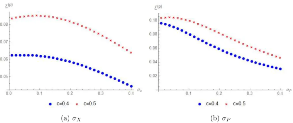
(7) 131 131 Substituting (3.23) into (3.21) yields:. \gam a_{3}A_{3}[\frac{\gam a_{3}-1{(\gam a_{3}-\alpha)\alpha}\frac{1}B}] ^{\frac{\gam a_{3}-1{\alpha-1}p^{\eta_{3}+\frac{\gam a_{3}-1{\alpha-1}+\frac {\alpha-1}{\gam a_{3}-\alpha}p=0. .. (3.25). To Satisfying the equality in hold (3.25) gives the following equations:. \eta_{3}+\frac{\gamma_{3}-1}{\alpha-1}=1 ,. (3.26). \gam a_{3}A_{3}[\frac{\gam a_{3}-1{(\gam a_{3}-\alpha)\alpha}\frac{1}B] ^{\frac{\gam a_{3}-1{\alpha-1}=\frac{\alpha-1}{\gam a_{3}-\alpha}. .. (3.27). It follows from (3.26) that we obtain:. \eta_{3}=\frac{\alpha-\gamma_{3} {\alpha-1} . 4. (3.28). Numerical Analysis. In this section, we calculate the four unknowns, A_{3}, \underline{y}(p), \gamma_{3} , and \eta_{3} , and investigate the effects of changes in the parameters on the threshold, \underline{y}(p) . The basic parameter values are set out as follows:. r=0.05, \delta=0.1, \mu x=0.01, \sigma_{X}=0.2, \mu_{P}=0.01, \sigma_{P}=0.2, \rho=0.3, \alpha=0.4,. p=10 , and c=0.4 . Then, we obtain A_{3}=14.0086,. \underline{y}(p)=0.058602, \gamma_{3}=-0.232449 , and. \eta_{3}=-1.05408.. The results of the comparative static analysis of the threshold,. \underline{y}(p) , are shown in Figures. 3‐7. Note that the blue circle represents the result of comparative static analysis when the firm’s manager is ambiguity‐averse (c=0.4) , while the red cross represents the results of comparative static analysis when the firm’s manager is ambiguity‐neutral (c=0.5) in Figures 3‐7. Figure 2 shows how investment decision‐making is influenced by the manager’s attitude toward ambiguity,. c. . Figure 2 shows that the capital investment threshold,. \underline{y}(p) , is increasing. with . This means that if the firm’s manager is more ambiguity‐averse, capital investment is c. delayed. An ambiguity‐averse manager tends to hesitate to invest in capital in an ambiguous business environment. \underline{\ve }(p) 0 0 0 0 0 0. Figure 2: The effect of changing the ambiguity attitude parameter, Figure 3 shows the impact of volatility of both output demand, \sigma_{P} .. c. \sigma_{X}. , on the threshold. \underline{y}(p) .. , and the price of capital,. If the firm’s manager is ambiguity‐averse (c=0.4) , the threshold. \underline{y}(p) is decreasing in.
(8) 132 both volatilities. This means that investment is delayed when either volatility increases. This. is consistent with the standard result of real options analysis. Conversely, if the firm’s manager. (c=0.5) , the threshold \underline{y}(p) is initially increasing in both volatilities. However, beyond a certain level in each volatility (about \sigma_{X}=0.091 and \sigma_{P}=0.037 ), the is ambiguity‐neutral. thresholds start to decrease.. \underline{y}1p) \underline{y}(p) 0 0. 0 0 0 0. 0. 0. 0. ec=04 xc=0.5. (a). \bullet cM.4. (b). \sigma_{X}. x. ct.5. \sigma_{P}. Figure 3: The effect of changing the volatility of output demand and capital price, on the threshold. \underline{y}(p). \sigma_{X}. and. \sigma_{P},. .. Figure 4 shows the impact of the correlation between the two Brownian motions,. W_{t}^{X} and. W_{t}^{P} , on investment decision‐making. The investment threshold \underline{y}(p) is increasing with the correlation coefficient \rho.. \underline{v}lp). \bullet c=0.4 xc=05. Figure 4: The effect of changing the correlation coefficient between W_{t}^{X} and W_{t}^{P}, threshold. \rho ,. on the. \underline{y}(p) .. Figure 5 shows how investment decision‐making is influenced by the expected rate of change of both the output demand and the price of capital,. \mu_{X}. and. \mu_{P} .. The investment threshold. \underline{y}(p). is increasing in both the expected rates of change. This implies that investment is hastened.
(9) 133 when the expected rate of change of the output demand and the price of capital is increasing.. \underline{v}(p). \bullet c=0.4 xc=0.5. (a). \bullet cM.4 xc=0.5. 5. (b). \mu_{X}. \mu_{P}. Figure 5: The effect of changing the drift coefficient of output demand and the price of capital, \mu_{X}. and. \mu_{P} ,. on the threshold. \underline{y}(p) .. Figure 6 shows the impact of the output elasticity of capital, making. Recall that output per unit of capital increases in. \alpha. \alpha. , on investment decision‐. . Figure 6 shows that the threshold. \underline{y}(p) is initially increasing with the output elasticity of capital. However, beyond a certain level (about. \alpha=0.3586. if. c=0.4 ,. and. \alpha=0.3759. if. c=0.5 ),. the threshold starts to decrease.. \underline{v}lp) 0. 0. 0. 0. \bullet c=04 Kc=05. Figure 6: The effect of changing the output elasticity of capital,. \alpha. , on the threshold. \underline{y}(p) .. Figure 7 shows how the price of capital affects investment decision‐making. Figure 7 shows that the threshold. \underline{y}(p) decreases as the price of capital decreases. This implies that a higher. price of capital delays investment. These results provide useful insights into investment decision‐making when output demand and the price of capital are ambiguous..
(10) 134 when the expected rate of change of the output demand and the price of capital is increasing.. \underline{v}(p). \bullet c=0.4 xc=0.5. (a). \bullet cM.4 xc=0.5. 5. (b). \mu_{X}. \mu_{P}. Figure 5: The effect of changing the drift coefficient of output demand and the price of capital, \mu_{X}. and. \mu_{P} ,. on the threshold. \underline{y}(p) .. Figure 6 shows the impact of the output elasticity of capital, making. Recall that output per unit of capital increases in. \alpha. \alpha. , on investment decision‐. . Figure 6 shows that the threshold. \underline{y}(p) is initially increasing with the output elasticity of capital. However, beyond a certain level (about. \alpha=0.3586. if. c=0.4 ,. and. \alpha=0.3759. if. c=0.5 ),. the threshold starts to decrease.. \underline{v}lp) 0. 0. 0. 0. \bullet c=04 Kc=05. Figure 6: The effect of changing the output elasticity of capital,. \alpha. , on the threshold. \underline{y}(p) .. Figure 7 shows how the price of capital affects investment decision‐making. Figure 7 shows that the threshold. \underline{y}(p) decreases as the price of capital decreases. This implies that a higher. price of capital delays investment. These results provide useful insights into investment decision‐making when output demand and the price of capital are ambiguous..
(11) 135 Camerer, C. and M. Weber, (1992). Recent developments in modeling preferences: uncertainty and ambiguity, Journal of Risk and Uncertainty, 5(4), 325‐370. Chen, Z. and L. Epstein, (2002). Ambiguity, risk, and asset returns in continuous time, Econo‐. metrica, 70(4), 1403‐1443. Dixit, A. and R. S. Pindyck, (1994). Investment under uncertainty, Princeton University Press, New Jersey, USA.. Dumas, B., (1991). Super contact and related optimality conditions, Journal of Economic Dy‐ namics and Control 15(4), 675‐685. Etner, J., M. Jeleva, and J.‐M. Tallon, (2012). Decision theory under ambiguity, Journal of Economic Surveys, 26(2), 234‐270. Guidolin, M. and F. Rinaldi, (2013). Ambiguity in asset pricing and portfolio choice: A review of the literature, Theory Decision, 74(2), 183‐217. Hartman, R., (1972). The effects of price and cost uncertainty on investment, Journal of Eco‐ nomic Theory, 5(2), 258‐266. Kast, R. and A. Lapied, (2010). Dynamically consistent Choquet random walk and real invest‐ ments, Working Paper LAMETA, DR 2010‐21.. Kast, R., A. Lapied, and D. Roubaud, (2014). Modeling under ambiguity with dynamically consistent Choquet random walks and Choquet‐Brownian motions, Economic Modelling, 38, 495‐503.. McDonald, R., and D. Siegel, (1986). The value of waiting to invest. The Quarterly Journal of Economics, 101(4), 707‐727. Nishimura, K. G. and H. Ozaki., (2007). Irreversible investment and Knightian uncertainty, Journal of Economic Theory, 136(1), 668‐694.. Stokey, N. L. (2009). The Economics of Inaction: Stochastic Control models with fixed costs. Princeton University Press.. Thijssen, J. J., (2011) Incomplete markets, ambiguity, and irreversible investment, Journal of Economic Dynamics and Control 35(6), 909‐921. Trojanowska, M. and P. M. Kort, (2010). The worst case for real options, Journal of optimization Theory and Applications, 146(3), 709‐734. Tsujimura, M., (2017) Partially Reversible Capital Investment under Demand Ambiguity. forth‐ coming in RIMS Kôkyûroku.. Wang, Z., (2010). Irreversible investment of the risk‐ and uncertainty‐averse DM under k‐ ignorance: The role of BSDE, Annals of Economics and Finance, 11(2), 313‐335..
(12) 136. Faculty of Commerce, Doshisha University Kamigyo‐ku, Kyoto, 602‐8580 Japan. E‐mail address: [email protected].
(13)
図


+2

関連したドキュメント
そして8件(フィリピン San Roque ,カタール Messaied , UAE Taweelah A 2,米国 MSE ,バハ マ GBPC ,ジャマイカ JPS ,トリニダード・ト バゴ Power Gen
Two grid diagrams of the same link can be obtained from each other by a finite sequence of the following elementary moves.. • stabilization
An idea to use frequency-domain methods and certain pseudodifferential operators for parametrization of control systems of more general systems is pointed
Standard domino tableaux have already been considered by many authors [33], [6], [34], [8], [1], but, to the best of our knowledge, the expression of the
Many authors argue that as the investment horizon increases, an investment portfolio with a higher proportion of assets will dominate, or will be preferred over a portfolio
H ernández , Positive and free boundary solutions to singular nonlinear elliptic problems with absorption; An overview and open problems, in: Proceedings of the Variational
We investigated a financial system that describes the development of interest rate, investment demand and price index. By performing computations on focus quantities using the
Schmidli, “Asymptotics of ruin probabilities for risk processes under optimal reinsurance and investment policies: the large claim case,” Queueing Systems, vol. Zhang, “Some results
