A Numerical Scheme for the Hele‑Shaw Problem in Oscillating Media
著者 イルマ パルピ
著者別表示 Irma Palupi journal or
publication title
博士論文要旨Abstract 学位授与番号 13301甲第4815号
学位名 博士(理学)
学位授与年月日 2018‑09‑26
URL http://hdl.handle.net/2297/00053027
Creative Commons : 表示 ‑ 非営利 ‑ 改変禁止 http://creativecommons.org/licenses/by‑nc‑nd/3.0/deed.ja
Doctoral Thesis
A Numerical Scheme for the Hele-Shaw Problem in Oscillating Media
Author:
Irma Palupi
Supervisor:
Prof. Seiro Omata
A thesis submitted in fulfilment of the requirements for the degree of Doctor of Science
in the
Division of Mathematical and Physical Sciences Graduate School of Natural Sciences And Technology
2018
Abstract
We study the Hele-Shaw problem in oscillating media, and mainly are interested in the
averaging behavior of the free boundary velocity, that is a homogenization problem. Our
focus is only on the one-phase Hele-Shaw problem neglecting the surface tension. A
general formula for the homogenized velocity is unknown. Current results are known for
the media periodic only in space or only in time. In this work, we develop an efficient
numerical scheme to estimate the averaging velocity in two dimensions with periodic
coefficients in both space and time. Also for comparison, we implement the regular finite
difference to obtain a numerical solution and we describe how to get a free boundary
position. We present several computation experiments to test the error of both for the
numerical solution and the free boundary position.
1 Introduction
In many years, Hele-Shaw problem have become one of popular model in fluid me- chanics. For two dimensions case, this is a popular model for pressure driven flow of an incompressible liquid between two parallel plates, names Hele-Shaw cell. And for three dimensions case, this is a model for pressure driven flow of an incompressible liquid in porous medium. In this work, we study the Hele-Shaw problem in oscillating media, and mainly are interested in the averaging behavior of free boundary velocity, i.e homogenization problem. Our focus is only on One-phase Hele-Shaw problem neglecting surface tension. One can simply represent this problem is flowing a liquid through the valleys area containing air only. For general periodic media, the homogenized solution is unknown. Current results have been revealed for the media that periodic only either in space or in time. We develop a numerical schemes to estimate the homogenized solution of normal velocity in Hele-Shaw problem with periodic coefficients in both space and time. Instead of directly solving the problem, we use the fact that One-phase Hele-Shaw problem is a zero heat specific limit of One-phase Stefan problem, then consider the equation in the enthalpy form. We implement the efficient numerical scheme, namely BBR method to solve the PDE, and use the idea in 1D case to estimate the average velocity r(q) in two dimensions.
2 Problem Statement
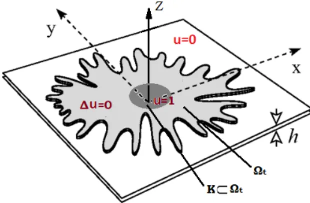
Suppose the Hele-Shaw problem is in R n , n = 2. Given Ω 0 as an initial domain, closed subset K ⊂ Ω 0 , with Ω 0 ⊂ Ω t , t > 0 is increasing. We want to find a pair of u(x, t) and free boundary ∂Ω t that satisfying (HS).
∆u(x, t) = 0 for (x, t) ∈ (Ω t \ K) × [0, ∞) u t = g(x, t)|∇u| 2 , for(x, t) ∈ ∂Ω t × (0, ∞) u(x, t) = 1 for(x, t) ∈ K × (0, ∞)
u(x, t) = 0 for(x, t) ∈ (R n \ Ω t ) × (0, ∞)
(HS)
Solution u(x, t) represents pressure of some viscous fluid that is injected into the air as in Figure HS. Neglecting surface tension, the area with air is assumed to have zero pressure on ∂Ω t , and function g(x,t) 1 represents the depth of hole at the free boundary that the liquid must fill while it is advancing. In fact, (HS) can be approximated by limiting specific heat coefficient c −→ 0 in the One-phase Stefan problem. The form of the One-phase Stefan problem is only distinguished by replacing the Laplace operator on (HS) with Heat operator with heat specific coefficient c > 0.
cu t − ∆u(x, t) = 0
4
Figure 1: Hele-Shaw cell for problem (HS)
On the Stefan problem, the solution of u models the temperature diffusion in ice melting, where the temperature in the ice region is preserved to be 0 o C. Here, −1 g is specified to be a latent energy in the phase transition solid to liquid. Then for numerical scheme, we rewrite the Stefan problem into the enthalpy formulation as written in (SF2).
cu t − ∆h(u) = 0 in ( R n \ K) × (0, ∞)
u = 1 in K × (0, ∞)
u(·, 0) = u 0 in R n
(SF2)
Operator h(u) = u + , where implicitly revealing (Ω t \ K ) := {x|u(x, t) > 0}.
2.1 Homogenization Problem
Suppose that the Hele-shaw cell in the periodic media is given by the problem to find u = u(x, t), Ω ⊂ R n × [0, ∞), (Ω(t) : {x|(x, t) ∈ Ω}) such that:
∆u(·, t) = 0 in Ω(t) \ K, t > 0 V (x, t) = g( x , t )|∇u(x, t)| x ∈ ∂Ω(t), t > 0 Ω(0) = Ω 0
u = h on K
u = 0 on ∂Ω(t), t > 0
(2.1)
for given h > 0, and g > 0 1-periodic function (g(x + k, t + l) = g(x, t), k ∈ Z N , l ∈ Z N ).
The homogenized problem of (2.1) has almost the same form except on the formula for the
normal velocity. Let u denotes the solution of (2.1) for any specific . In Pozar (2015),
there exist r = r(q), r : R N 7→ [0, ∞) depending only on g such that u → u, Ω → Ω as
→ 0, where (u, Ω) is the solution of (2.1) with V (x, t) = r(∇u(x, t)). In general, r(q)
has no explicit form. However, in special cases we know the following formula for r(q).
• If g = g(t) depends only on t, then r(q) = hgi|q|, where hgi = R 1
0 g(τ )dτ is the average of g.
• If g = g(x) depends only on x, then r(q) = h 1
1g
i |q|, where h 1 g i = R 1
0 1
g(τ) dτ is the average of 1 g .
If g depends on both x and t, the explicit form of r(q) is not known in general, and can appear to be complicated. The number of r(q) is related to Poincare’s rotation number.
Nonethelesss, for particular case of q, it is interesting to observe the existence of the interval where velocity becoming constant, namely pinning interval.
Lemma 2.1. Suppose that g(x, t) = f (x + t) where f = f (x) is a positive periodic continuous function. Then r(q) = 1 for q ∈ [ max 1 f , min 1 f ].
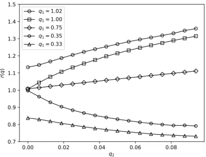
Figure 2: graph of r(q) in 1D for g(x, t) = sin(2π(x + t))
2+ 1/2 pinning interval is shown for constant r(q) = 1 in [2/3, 2]
However in the higher dimension, if function g is time-independent, homogenized solution convergence to r(q) = h 1
1g
i |q| , the same as in 1-D case. Also for simple scaling argument, it shows that solution homogenization with g = g(t) converge to r(q) = hgi|q|.
2.2 Estimating The Average Normal Velocity
To estimate the average normal velocity in 2D, we are motivated by the idea in 1D case, where the homogenized problem can be simplified to the ODE
( (y ε ) 0 (t) = g( y
εε (t) , t ε )|q|, t > 0,
y ε (0) = y 0 , (ODE)
and the solution y ε converge locally uniformly as ε → 0+ to the solution of linear ODE.
( y 0 (t) = r(q), t > 0,
y(0) = y 0 ,
6
Therefore, we can estimate r(q) in 1D by solving (3.3) for a small ε > 0.
r(q) = y(1) − y 0 ≈ y ε (1) − y 0 .
Or by scaling argument, fix ε = 1 and solve (3.3) for a large time T 1.
r(q) = y(T ) − y 0
T ≈ y 1 (T ) − y 0
T .
x 2
x 1
L 1
∂Ω 0
Ω 0
∂Ω ε t
∂β(z)
∂x
1= q 1 Ω ε t
Figure 3: The setting of initial condition in 2D case to estimate the value of r(q).
By the convergence in the Hausdorff distance, we see that T ε → L
1r(q) −L
0as ε → 0. This allows us to estimate r(q) by choosing 0 < ε 1 and using
r(q) ≈ L 1 − L 0
T ε .
3 Numerical Method
3.1 Explicit Finite Difference Method
For two dimension case, the numerical scheme of explicit finite difference for problem (SF2) can be written as (3.1),
u k+1 i,j = u k i,j +
∆t c∆x 2
{h(u k i−1,j )
+ h(u k i+1,j ) − 4h(u k i,j ) + h(u k i,j+1 ) + h(u k i,j−1 )}
(3.1)
with stability condition as the follows.
∆t c∆x 2 < 1
2 . (3.2)
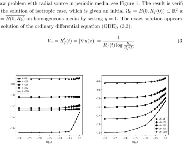
The explicit finite difference method is implemented to obtain numeric solution of Hele- Shaw problem with radial source in periodic media, see Figure 1. The result is verified to the solution of isotropic case, which is given an initial Ω 0 = B(0, R f (0)) ⊂ R 2 and K = B(0, R k ) on homogeneous media by setting g = 1. The exact solution appears to be solution of the ordinary differential equation (ODE), (3.3).
V n = R 0 f (t) = |∇u(x)| = 1 R f (t) log R R
kf
(t)
(3.3)
3.0 2.5 2.0 1.5 1.0 0.5 0.0
log
10c 1.6
1.4 1.2 1.0 0.8
M=64 M=128 M=256 M=512 M=1024
3.0 2.5 2.0 1.5 1.0 0.5 0.0
log
10c 1.8
1.6 1.4 1.2 1.0 0.8 0.6
M=64 M=128 M=256 M=512 M=1024
Figure 4: Maximum absolute error of solution with x-axis
Explicit finite different is very restricted to the stability condition. The reasonable small parameter of specific heat and acceptable mesh size compare to coefficient periodic, even lead to the computation much slower. Therefore, we do not recommend this method for numeric solution homogenization in 2D.
3.2 BBR Scheme as Implicit Method
Since the explicit method restrict the computation with the stability condition and
the reasonable size of M for the coefficient period , we provide an efficient numerical
scheme firstly introduced by Berger, Br´ ezis and Rogers (1979) and the further studied by
Murakawa(2011) for the the types of non-linear equation such a (SF2). We refer to this
scheme as BBR scheme. Choosing a time step ∆t > 0, we iteratively find the sequences
8
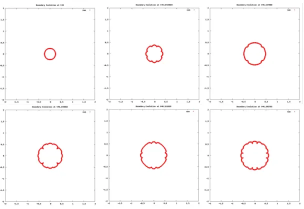
Figure 5: Numeric free boundary by explicit method for a given initial open ball domain with periodic function g(x, t) > 0
.
u k k≥1 ,
z k k≥0 of solutions of
cµ k−1 u k − τ ∆u k = cµ k−1 β(z k−1 ) in U,
∂u k
∂x 1
(0, ·) = q 1 , u k (1, ·) = 0,
u k 1-periodic in x 2 ,
(3.4a)
z k = z k−1 + µ k−1 (u − β(z k−1 )) − τ c
∂
∂t 1 g ε
(·, t k−
12
![Figure 2: graph of r(q) in 1D for g(x, t) = sin(2π(x + t)) 2 + 1/2 pinning interval is shown for constant r(q) = 1 in [2/3, 2]](https://thumb-ap.123doks.com/thumbv2/123deta/5642294.2003601/6.893.218.763.323.694/figure-graph-d-sin-pinning-interval-shown-constant.webp)