in Oscillating Media
著者 イルマ パルピ
著者別表示 Irma Palupi journal or
publication title
博士論文本文Full 学位授与番号 13301甲第4815号
学位名 博士(理学)
学位授与年月日 2018‑09‑26
URL http://hdl.handle.net/2297/00053028
Creative Commons : 表示 ‑ 非営利 ‑ 改変禁止 http://creativecommons.org/licenses/by‑nc‑nd/3.0/deed.ja
A Numerical Scheme for the Hele-Shaw Problem in Oscillating
Media
Graduate School of Natural Sciences And Technology Kanazawa University
Division of Mathematical and Physical Sciences
Student ID No. : 1524012011 Name : Irma Palupi
Chief Advisor : Prof. Seiro Omata
Date of Submission : June 29, 2018
We study the Hele-Shaw problem in oscillating media, and mainly are interested in the averaging behavior of the free boundary velocity, that is a homogenization problem. Our focus is only on the one-phase Hele-Shaw problem neglecting the surface tension. A general formula for the homogenized velocity is unknown.
Current results are known for the media periodic only in space or only in time.
In this work, we develop an efficient numerical scheme to estimate the averaging
velocity in two dimensions with periodic coefficients in both space and time. Also
for comparison, we implement the regular finite difference to obtain a numerical
solution and we describe how to get a free boundary position. We present several
computation experiments to test the error of both for the numerical solution and
the free boundary position.
I would like to express my sincere gratitude for my chief supervisor, Professor Seiro Omata for his continuous support during my study at Kanazawa University. I also would like to express my deep gratitude to Assistant Professor Norbert Poˇ z´ ar for his patience and guidance during my research work. I thank for every opportunity to learn at Kanazawa University, to join the interesting courses and to attend the special lectures held by Department of Mathematical and Physical Sciences which give me a new sight for the field that I am interested in. I also thank the doctoral program for the development of Global Human Resources in Mathematical and Physical Sciences (GHR program) with support from Ministry of Education, Culture, Sports, Science, and Technology (MEXT) for the generous opportunity to be part of the program. My Deep appreciation is also for all members of Omata laboratory and Japan Indonesian Student Community (PPI) in Kanazawa for their help and the life suggestions, especially at the beginning of living in this town.
Finally, I wish to thank my parents for their love, supports, and encouragements in my entire life. Thank you for never giving up to strengthen me to believe.
ii
Abstract i
Acknowledgements ii
Contents iii
List of Figures v
Abbreviations vii
1 Introduction 1
1.1 Introduction . . . . 1
1.2 Content of the thesis . . . . 4
2 Hele-Shaw Problem 6 2.1 Physical Phenomena . . . . 6
2.1.1 Governing Equation for Hele-Shaw Flow . . . . 7
2.1.2 Hele-shaw Problem as a limit of Stefan Problem . . . . 9
2.2 Homogenized Hele-Shaw Problem . . . . 11
2.2.1 Homogenized Hele-Shaw Problem . . . . 12
2.2.2 Homogenized Problem in 1-D . . . . 14
2.3 Homogenization in 2-D . . . . 16
3 Stefan Problem 22 3.1 Stefan Problem . . . . 22
3.1.1 Enthalpy Formulation . . . . 24
3.1.2 Normal Velocity Derivation . . . . 25
4 Explicit Methods and Implementation 30 4.1 Explicit Finite Difference Method . . . . 30
4.1.1 Discretization Scheme for One Dimensional Case . . . . 30
4.1.1.1 Numerical Scheme . . . . 31
4.1.1.2 Adjusting Free Boundary Position . . . . 31
4.1.2 The scheme for Two Dimensional Case . . . . 32
4.1.2.1 Numerical Scheme . . . . 32
iii
4.1.2.2 Adjusting Numeric Free Boundary in 2D Cartesian
Grid . . . . 33
4.2 Numerical Results and Discussion . . . . 33
4.2.1 One Dimensional Case . . . . 33
4.2.1.1 Numerical Solution . . . . 34
4.2.1.2 Numerical Error of Solution and Free Boundary Position . . . . 35
4.2.2 Two Dimensional case . . . . 36
4.2.2.1 Numerical Solution in Periodic Media . . . . 37
5 BBR Scheme as an Efficient Method 41 6 Multigrid Method 44 6.1 Multigrid . . . . 44
7 Numerical Implementation for Hele-shaw Problem 49 7.1 Application of the multigrid solver to the BBR scheme . . . . 49
7.2 Estimating Error caused by non-periodic g . . . . 49
7.3 General direction . . . . 51
7.4 Numerical results . . . . 52
7.4.1 Discussion . . . . 53
Bibliography 59
1.1 Hele-Shaw cell experiment (Pozar, 2018. Used with permission.). . . 2
2.1 Hele-Shaw cell for problem (HS) . . . . 10
2.2 Sample r(q) in one dimension for g(x, t) = sin(2π(x + t)) + sin(2π(x + 3t)) + 3. Note the pinning intervals at speeds 2k − 1 for k = 1, 2, . . . , 5. 16 2.3 Free boundary position of homogenized problem with g(x, t) = g(t). 16 2.4 Free boundary position of homogenized problem with g(x, t) = g(x). 17 2.5 Neumann problem (6.1.1) in 2D case to estimate the value of r(q). . 18
4.1 Extrapolation to estimate ¯ x
f. . . . 32
4.2 Boundary lies on the Cartesian grid between a 5-point stencil . . . . 33
4.3 Free Boundary Position and its absolute error . . . . 34
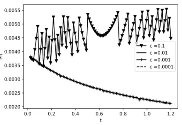
4.4 Maximum error of Solution in time, with ∆x = 0.004 and = 0.0001 35 4.5 Error of numerical solution in the logarithmic scale. . . . 36
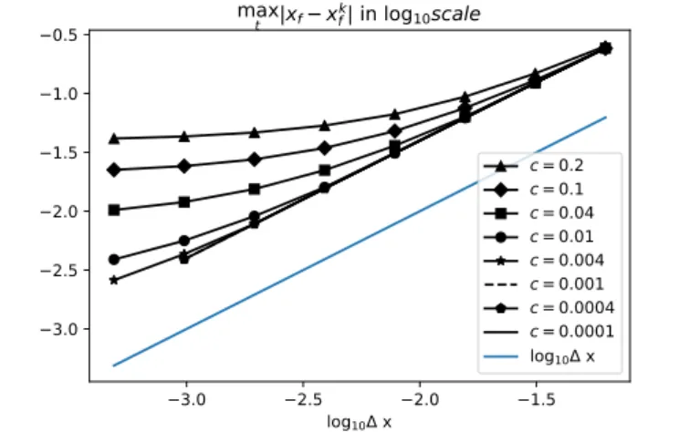
4.6 Error of numeric free Boundary Position in the logarithmic scale. . 36
4.7 Maximum absolute error of solution with x-axis . . . . 37
4.8 Maximum absolute error of free boundary with x-axis . . . . 38
4.9 Maximum absolute error of solution with x-axis . . . . 38
4.10 Error behavior for g(x, t) = sin(
2x−t0.1) . . . . 39
4.11 Error behavior for g(x, t) = sin(
2x−t0.01) . . . . 39
4.12 Error behavior for g(x, t) = sin(
2x−t0.001) . . . . 40
6.1 Transfer between grids, restriction and prolongation. . . . . 45
7.1 (Top) The contour plot of r(q) with g(x, t) = sin(2π(x
1+ t)) + 2. The pinning interval [
13, 1] × {0} is apparent, see Lemma 2.2.1, where the average velocity is pinned to 1. The solid contours were obtained with M = 256, while the dotted contours were obtained with M = 128. (Bottom) Detail of the pinning interval computed with M = 512. . . . 55
7.2 Values of r(q), q = (q
1, q
2), for g(x, t) = sin(2π(x + t)) + 2 with M = 1024 as a function of q
2for several chosen of q
1. . . . 55
v
7.3 (Top) Contour plot of r(q) with g(x, t) = sin(2π(x
1+t))+sin(2π(x
2+ t)) + 3 and M = 256. As expected, pinning intervals appear in directions (1, 0) and (0, 1), however, there is also a visible pinning interval in direction (1, 1) where the velocity appears to be pinned to √
2. The plot is symmetric with respect to the reflection across the direction (1, 1). (Bottom) Detail with M = 1024 around the pinning interval with velocity √
2. There might be other pinning intervals nearby. The small squares along the diagonal are artifacts of contour reconstruction. . . . . 56 7.4 Contour plot of r(q) with g (x, t) = sin(2π(x
1+t))+sin(2π(x
1+3t))+3
computed with M = 256. The two visible pinning intervals along the q
1axis where the velocity is pinned to 1 and 3. . . . . 57 7.5 Contour plot of r(q) with g(x, t) =
12cos(2πt)(sin(2πx
1)+sin(2πx
2))+
2 with M = 256. Pinning intervals appear in the directions of (1, 0), (−1, 0), (0, 1) and (0, −1) (the plot is symmetric with respect to the
rotation by
π2). . . . . 57 7.6 (Top) The free boundary of the numerical solution of the Hele-Shaw
problem with a given source f = 1500 max{0.1 − |x − (
12,
12)|, 0}
and a function g(x, t) = sin(2π(x
1+ t)) + 1.05 with initial data Ω
0=
x : |x − (
12,
12)| < 0.1 . The free boundary is plotted at times
t = 0.02m, m ∈ N . A facet seems to appear in direction (1, 0). It
reaches its maximum length at t ≈ 0.12. Solid line is the solution
with M = 8192, ε =
5121, while the dotted line is with M = 2048,
ε =
1281. We used 1 V-cycle. (Bottom) Detail of the region with facets. 58
HS Hele Shaw SF Stef an Problem BBR Berger Br´ ezis Rogers SOR Successive OverRelaxation
vii
Introduction
1.1 Introduction
Patterns in nature have been of interest for many years in various fields of science.
They appear in numerous natural phenomena that have an order or repeated systematic structure. Scientists want to capture them in their models to understand the rules of their formulation. Interestingly, different natural phenomena may have similar pattern. For instance, the pattern in branching of a tree look similar to the ice crystallization, dendritic copper, and the burned wet pine if the electricity is run between two nails sunk into it, and also to the flow of viscous fluid.
Particularly in the fluid mechanics, researches studying a pattern of a flow in order to learn various of its behavior, such as abnormality, direction, strength, etc. In fluids, the patterns are usually caused by instabilities. For example in the interaction of two fluids, Rayleigh-Taylor instability shows a mushroom-like pattern as an indication of mixing two different densities of the fluids. There is also an instability caused by the difference between tangential velocities of fluids that shows as a triangle-wave pattern forms a cloud-like shape. The example study of such instabilities can be found in the Saffman-Taylor instability. They
1
discovered a finger-like pattern on the interface in between fluids with different viscosities, called viscous fingering. They observed such a pattern in the porous medium and Hele-shaw cell [1]. Hele-Shaw cell is an experiment invented by Henry Selby Hele-Shaw. It presents a fluid flow through a narrow gap between parallel plates, which for many years was used as a model to approximate various problems of viscous fluid in fluid mechanics.
Furthermore, a pattern occurs in two different types of geometry, radial and rectangular. Viscous fingering in a rectangular geometry refers to the Hele-Shaw cell with a less viscous fluid injected continuously from one end of the cell. In this situation, the interface is transported by the gradient of pressure (sufficiently high) through a more viscous area and an instability occurs which forms a finger-like pattern on the interface. The interface is initially flat. Once the pressure drives to the more viscous part, the interface starts to show a single finger where the gradient is locally highest at the tip. After some time the tip will turn blunt, then split into a branch of fingers. Each finger on the branch growths independently.
Figure 1.1: Hele-Shaw cell experiment (Pozar, 2018. Used with permission.).
On the other hand, radial viscous fingering occurs when injecting a Hele-Shaw cell through a source point in the middle of the plates. Initially, the interface is given by a circle, then it spreads and splits turning into radial fingering pattern.
Unlike in the rectangular fingering, there is no such single finger appearance in
radial geometry. Once the interface becomes unstable, it will turn into radial
fingering-look. This pattern also looks familiar with a typical pattern in bacteria
growth, crystal growth, and tumor growth for instance. Hele-shaw problem appears in many fields area. It is an example of non-linear diffusion phenomena. Many industry fields implement the Hele-shaw model to approximate the real situation in their sector, for example, a molding process in the plastic industry [2], petroleum extraction in the oil industry, and many other examples.
In many years, Hele-Shaw problems have been one of popular model in fluid mechanics. Researchers in porous media and the flow in between two parallel plates consider this problem as a reliable model. In this work, we study the Hele-Shaw problem in oscillating media, and mainly are interested in the averaging behavior of the free boundary velocity, namely the homogenization problem. Our focus is only on the one-phase Hele-Shaw problem neglecting surface tension.
One can merely represent this problem as a flow of a liquid through the valleys area, and we are interested in the homogenized behavior of the free boundary.
For a general type of media, the homogenized solution for Hele-Shaw is unknown.
Current results know only for the media that periodic only in space or only in time [3]. We recently developed a numerical scheme to estimate the homogenized normal velocity in the Hele-Shaw problem with periodic coefficients in both space and time, see [4].
The homogenization method has many important practical implementations in
material sciences since the macroscopic appearance are mostly used in industry. It
comes from the fact that the macroscopic appearance has better characteristics
in a practical industry than the microscopic point of view. In the microscopic
appearance, there will appear the heterogeneities that become a source of error
such that computationally it is difficult to be implemented. Therefore the theory
of homogenization which describes the behavior of a composite material from the
local characteristics of the heterogeneities answering the difficulties.
Instead of directly solving the problem, using the fact that the Hele-Shaw problem can be described as the zero specific heat limit of the one-phase Stefan problem, we consider a Stefan problem in enthalpy formulation to solve the problem. Since the Stefan equation is a nonlinear equation, we must find a method that reduces the nonlinearity so that we perform the computation significantly faster than the explicit finite difference scheme. We use the method firstly developed by Berger, Br´ ezis, and Rogers in [5] to solve a similar nonlinear homogeneous problem. We will refer to it as the BBR method. As it uses an implicit scheme, it is also essential to choose an efficient numerical method to solve the implicit scheme. It turns out that a multigrid scheme for the linear elliptic problem works well even though there is a jump across the free boundary.
1.2 Content of the thesis
We are interested in developing a numerical method to efficiently compute the numerical solution of Hele-Shaw problem for both Dirichlet and Neumann boundary data. Furthermore, we apply the method to approximate a numerical solution of a homogenized problem of a given media that are periodic both in space and time, and moreover to observe the homogenized velocity in such periodic media. The content of the thesis is as follows. In chapter 2, we brief the formulation of the governing equation for the Hele-shaw problem and the homogenization problem.
We explain current results for averaging free boundary velocity if the media depends only on time or only on space. The idea to approximate the average normal velocity for general direction in 2D is adapted from the one specific direction case only.
In chapter 3, we explain the consideration of indirectly solving the Hele-Shaw
problem via the Stefan problem in the enthalpy formulation. Here, we consider
two problems, the problem with source spreading from the middle of the area
of the plate (Dirichlet boundary data), and a Neumann problem. In chapter 4,
explicit finite difference scheme is explained to obtain a numerical solution in
both one dimension and two dimensions, especially how to approximate the free
boundary. We also make several observations of the numerical solution. In chapter
5, we explain the advanced implicit method to solve the equation in the enthalpy
form, which we call the BBR scheme. In chapter 6, we describe how does the
Multigrid linear solver is adapted to our problem. Finally, in chapter 7, we give
the implementation of the BBR scheme to estimate the free boundary velocity in
two dimensions. Several interesting results are shown in this chapter.
Hele-Shaw Problem
2.1 Physical Phenomena
In two dimensional case, Hele-shaw problem is a two dimensional model for the pressure-driven flow of viscous liquid throughout a very tiny gap of two plates with given boundary data on the source. This model has several applications, such as in electro-machining, injection molding, and even basic model for tumor growth, and many other industrial fields. Furthermore, in three-dimensional model Hele-Shaw problem appears in the porous medium, i.g pipe injection in the petroleum field. In the plastic molding process, in particular, it is useful to determine the end position of the melting plastic will be filling the mold, which is the circulation hole for the air to way out.
There are several more specific problem refer to this model. One-phase Hele-Shaw problem is usually describing the evolution of a liquid being injected into a Hele- shaw cell, and the free boundary problem occurs on the liquid surface against the air. Meanwhile, a two-phase Hele-shaw problem can be a model for free boundary problem of two liquids having a different viscosity. In three dimensional case, this model refers to the problem called porous medium equation. However, in this
6
research work, our interest is in the one-phase Hele-shaw problem in two dimensions with neglecting the effect of surface tension on the boundary.
2.1.1 Governing Equation for Hele-Shaw Flow
This work focus only on the scope of the Newtonian fluid. In fluid dynamics, Hele-Shaw flow is one of Stokes flow of a liquid that distributes through a very tiny space between two plates which continually injected by fluid from the source inside the fluid area. This phenomenon can be derived from conservation law of mass, where saying that a density changing per unit volume depend only on the flux passing through its boundary, either due to the absence of fluid transport or due to volume movement, and a given external source. It states that changing a mass
in the fixed domain V is proportional to a given flux q moves to the boundary of V in the normal direction, and a given external source contribution f (x, t).
d dt
Z
V
ρdV = Z
S
q · dS + Z
V
f(x, t)dV
= Z
V
∇ · qdV + Z
V
f(x, t)dV , by divergent theorem
⇔ ρ
t− ∇ · (q) = f(x, t) ,since fixed volume V.
(2.1.1)
Since the flux is caused by the difference of pressure u, q = −ρ∇u and no outer source, then from the we obtain,
ρ
t+ ∇(ρ∇u) = 0. (2.1.2)
We assume that the liquid is an incompressible fluid (e.g water), therefore it remains the following Laplace equation.
∆u = 0 (2.1.3)
In a Hele-Shaw cell, we consider the flow of a Newtonian viscous fluid that is incompressible, and driven by pressure caused by a constant given source in the middle of the cell. Hele-shaw problem can be derived from the equation for the motion of viscous fluid, i.e Navier-Stokes equation with neglecting the external body force. Suppose that Ω
tbe the diffuse region in coordinate (x, y) of a liquid at time t and 2h is a length of gap between the plates. Outside of diffuse region is filled only by the air and we assume has zero pressure u = 0. For h → 0, the velocity in the vertical direction z is parabolic and determining the constants so as to make the velocity q = 0 at z = ±h, so that it satisfies
q = − 1
2µ (h
2− z
2)∇u (2.1.4)
where µ is a fluid viscosity, such that the average of velocity over the gap is following
¯ q = 1
2h Z
h−h
qdz = − h
212µ ∇u. (2.1.5)
The average velocity ¯ q also satisfies the continue equation in 2D, such that it implies that the pressure u in Ω
tsatisfies Laplace equation
∆u = 0.
For the boundary condition on the free boundary ∂Ω
t, there are dynamic and kinetic boundary condition. The dynamic boundary condition occurs to be
u = 0 on ∂ Ω
t,
since we neglecting the surface tension. And for the kinematic boundary condition, the normal velocity of the fluid particles on the boundary satisfying
V
n= ¯ q · ν on ∂ Ω
t(2.1.6)
where ν is the unit outer normal vector on ∂Ω
t. Since u can be seen as a level set, (2.1.6) can be rewritten as
V
n= −k|∇u| = u
t|∇u| (2.1.7)
where k is a constant equals to −
12µh2.
2.1.2 Hele-shaw Problem as a limit of Stefan Problem
Suppose the Hele-Shaw problem is in R
n, n = 2. Given Ω
0as an initial domain for given initial data u
0, and K ⊂ Ω
0⊂ Ω
t, t > 0 be a closed subset. We want to find a pair of u(x, t) and free boundary ∂Ω
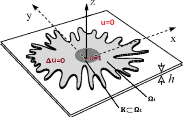
tthat satisfying (HS).
∆u(x, t) = 0 for (x, t) ∈ (Ω
t\ K) × (0, ∞) u
t= g(x, t)|∇u|
2, for(x, t) ∈ ∂Ω
t× (0, ∞) u(x, t) = 1 for(x, t) ∈ K × (0, ∞)
u(x, t) = 0 for(x, t) ∈ ( R
n\ Ω
t) × (0, ∞)
(HS)
Solution u(x, t) represents the pressure of some viscous fluid that is injected into
Hele-shaw cell. The area with no fluid is assumed to have zero pressure, and function
g(x, t) is a given continuous positive function, denoting media representation. As in
the original Hele-shaw problem, this function is some constant k which describing
a homogeneous structure of the media.
1gcan be representing a depth of the hole
Figure 2.1: Hele-Shaw cell for problem (HS)
must be filled by a liquid when evolving. This value change in the position and time.
If we look at the one-phase Stefan problem, the free boundary problem is similar except on the term first time derivative in the Stefan problem. The heat diffusion speed depends on the heat specific parameter c (see chapter 3), that is the quantity of heat required to change the temperature 1 degree celsius in one unit of mass.
As c → 0 the Stefan problem approaches the Hele-shaw problem, and as t → ∞ the temperature diffusion will reach the steady-state and no longer has the term first-time derivative. The work in [6] explains the asymptotic behavior of the solutions between two problems including the free boundaries as t → ∞. They explain the behavior in the aspect of the near-field limit and far-field limit. It states for 1 dimensional case when g(x, t) is constant both in x and t, the self-similar solution of two problems converge to the same constant as t → ∞ for every x > 0.
The convergence is not uniform. Despite the free boundary of both problem have the same growth rate √
t, the free boundary of the 1-D Stefan problem converge to Hele-Shaw when c → 0.
Different to the 1-D case, The solution of Stefan problem is not ultimately to be the Hele-shaw as t → ∞, for n >= 2 there is only the convergence behavior to a stationary state of both problem, and the asymptotic behavior is different.
Meanwhile, in 2 dimensions case, it shows that the Stefan problem simplifies to
the Hele-shaw. An unlikely 1-D case, the HS and SF problem for multidimensional spaces do not always have a classical solution. However, they always have a weak solution globally over time.
2.2 Homogenized Hele-Shaw Problem
Homogenization theory is concerned with the effects of rapidly varying coefficients to the solution of PDE. This problem appears in obtaining the macroscopic equation for the system with a fine microscopic structure for instance, which is to be our interest. Suppose that we have two different length scale of oscillation period in PDE respectively for macroscopic and microscopic structure, 1 and 0 < < 1. For fixed we have a solution u
for microscopic scale and u for the macroscopic, are different and complicated in general. Homogenization theory studies the limiting behavior of the solution of microscopic to the homogenized problem as → 0. The idea is the limit effects toward homogenized problem will be the averaged out of the fine-structure.
For example in a periodic homogenization of elliptic problem, we have quantity u satisfying the elliptic equation
−∇ · (A(x)∇u(x)) = f(x). (2.2.1)
The microscopic solution u
for fixed oscillation period satisfies
−∇ · (A( x
)∇u
(x)) = f (x). (2.2.2)
As → 0, we have u
→ u
h, where u
his solution satisfied the homogenized form
−∇ · (A
h∇u
h). (2.2.3)
Thus, homogenization problem are to find the asymptotic convergence of solution u
→ u
h, and to obtain the expression for A
hwhich is not simply the average of A(
x) in general.
However, for the Hele-shaw problem we are interested in the convergence as → 0 of the solution u
, and the structure of homogenized free boundary velocity. In the work of [7], they derive the explicit formula for homogenized free boundary velocity with function g = g(x) depends only on space variable, and establish the uniform convergence of the free boundary. Furthermore, [3] consider the homogenization in heterogeneous media both in space and time, and found that the free boundaries for various dependence of normal velocity converge locally uniformly in Hausdorff distance. It was also observed that non-periodic, fractal-like variations in the flow lead to anomalous diffusion in Stefan and Hele-Shaw problems [8].
2.2.1 Homogenized Hele-Shaw Problem
Suppose that the Hele-shaw cell in the periodic media is given by the problem to find u = u(x, t), Ω ⊂ R
n× [0, ∞), (Ω(t) : {x|(x, t) ∈ Ω}) such that:
∆u(·, t) = 0 in Ω(t) \ K, t > 0 V (x, t) = g(
x,
t)|∇u(x, t)| x ∈ ∂Ω(t), t > 0 Ω(0) = Ω
0u = h on K
u = 0 on ∂ Ω(t), t > 0
(2.2.4)
for given h > 0, and g > 0 1-periodic function (g(x + k, t + l) = g(x, t), k ∈ Z
N, l ∈
Z
N).
and for scale ε > 0 we introduce the rescaled g
ε(x, t) := g(
xε,
εt). Note that in general scaling g(ε
αx, ε
βt) is possible, but it leads to a simpler behavior than this critical scaling α = β, see for example [9]. Keeping all other parameters fixed, for every given ε > 0 we get a solution {Ω
εt}
t≥0, u
εof (2.2.4) with g = g
ε. The goal is to identify the homogenization limit ε → 0 of these solutions.
We shall denote
Ω = [
t≥0
Ω
t× {t} and Ω
ε:= [
t≥0
Ω
εt× {t}.
In [3], under certain regularity assumptions on the data K, Ω
0and g, it was proved that there exist limits {Ω
t}
t≥0and u such that u
ε→ u in the sense of half-relaxed limits and ∂Ω
ε→ ∂Ω in Hausdorff distance. Furthermore, the pair (Ω, u) is the unique solution of the homogenized problem in which Ω evolves with the normal free boundary velocity
V = r(∇u) x ∈ ∂Ω
t(2.2.5)
and u is again the solution of (HS), where r : R
n→ R is a nonnegative function that depends only on g.
A straightforward modification of the arguments in [3] shows the same homoge- nization result if the Dirichlet boundary condition on ∂K in (HS) is replaced by a Neumann boundary condition
∂u∂ν(·, t) = 1.
However, there does not seem to be any explicit formula for r(q), and it is not even
known whether r is continuous in general. It is only known that r
∗(a
1q) ≤ r
∗(a
2q)
for any 0 < a
1< a
2and any q ∈ R
n\ {0}, where r
∗and r
∗denote the upper and
lower semicontinuous envelopes of r, respectively. See [3] for more details. Formal
calculations indicate that r(q) is in general only
12-H¨ older continuous if g is smooth
and r(q) might be discontinuous if g is only H¨ older [10]. Our goal is to estimate
r(q) numerically. We are in particular interested whether the homogenized problem has solutions whose free boundary develops flat parts (facets ).
2.2.2 Homogenized Problem in 1-D
x u
εΩ
01
K
-q
Let K = (−∞, 0] and Ω
0= (−∞, 1), and we use the boundary condition u
x(0, t) = q on ∂K = {0} for some q < 0 in (HS). Then Ω
εt= (−∞, y
ε(t)) for some y
ε> 0.
The solution of Laplace’s equation is u
ε(x, t) = q(x − y
ε(t)) in this case. The free boundary velocity equation for Ω
εsimplifies to
(y
ε)
0(t) = g(
yεε(t),
tε)|q|, t > 0, y
ε(0) = 1,
(2.2.6)
which is a simple initial-value problem for an ordinary differential equation (ODE).
It is known, see [9, 11], that y
εconverges locally uniformly as ε → 0+ to the solution y of the ODE
y
0(t) = r(q), t > 0, y(0) = y
0,
where r : R → R depends only on g. This equation has the unique solution
y(t) = y
0+ tr(q). We can therefore estimate r(q) numerically by solving (2.2.6)
for a small ε > 0 and finding
r(q) = y(1) − y
0≈ y
ε(1) − y
0.
By a scaling argument, this can be shown equivalent to solving (2.2.6) with ε = 1 for a large time T 1 and then finding
r(q) = y(T ) − y
0T ≈ y
1(T ) − y
0T .
Since (2.2.6) can be efficiently solved numerically, we can estimate r(q) rather easily.
The actual form of r(q) is known only in certain cases [9]:
• g(x, t) = g(t): if g depends only on t, then r(q) = hgiq, where hgi = R
10
g(t) dt is the average of g.
• g(x, t) = g(x): if g depends only on x, then r(q) =
1h
1gi q, where D
1 g
E
= R
10 1
g(x)
dx is the average of
1g.
If g depends on both x and t nontrivially, the explicit form of r(q) is not known and in fact it can be very complicated, see Figure 2.2 for an example. The number r(q) is related to Poincar´ e’s rotation number.
Nonetheless, we can still find the value of r(q) at least for particular q. Particularly interesting is the existence of intervals of constant velocity, which we call pinning intervals. See also [10] for a related problem on a droplet motion.
Lemma 2.2.1. Suppose that g(x, t) = f(x−t) where f = f(x) is a positive periodic continuous function. Then r(q) = 1 for q ∈ [−
min1f, −
max1 f].
Proof. Let L > 0 be a period of f . Fix q ∈ [−
min1f, −
maxf1]. Since
|q|1∈
[min f, max f ], there exists ξ ∈ R such that f(x
0) =
|q|1for all x
0∈ ξ + L Z .
0 1 2 3 4 q
0 2 4 6 8 10
r(q )
Figure 2.2: Sample r(q) in one dimension for g(x, t) = sin(2π(x+t))+sin(2π(x+
3t)) + 3. Note the pinning intervals at speeds 2k − 1 for k = 1, 2, . . . , 5.
But y
ε(t) = εx
0+ t is then a solution of (2.2.6) for any x
0∈ ξ + L Z and ε > 0. By uniqueness of (2.2.6) (comparison principle), we conclude that
yε(T)−yT ε(0)= 1 for any ε > 0 and therefore r(q) = 1.
Figure 2.3: Free boundary position of homogenized problem with g(x, t) = g(t).
2.3 Homogenization in 2-D
The shape of the free boundary ∂ Ω
εis in general not simple in two dimensions and
therefore the solution of (HS) is not a linear function anymore. We therefore have
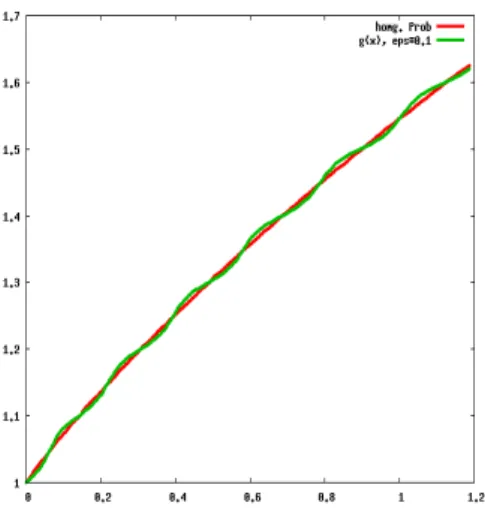
Figure 2.4: Free boundary position of homogenized problem with g(x, t) = g(x).
to solve the full problem to estimate r(q). We first observe that for a given q ∈ R
nthe moving plane
P
q(x, t) := |q|
r(q)t − x · q
|q|
x ∈ R
n, t ∈ R , Ω
q,t:= {x : P
q(x, t) > 0} =
x : x · q
|q| < r(q)t
is a solution of the homogenized problem (2.2.5).
Let us suppose that q = (q
1, 0) for some q
1< 0. We consider the Hele-Shaw problem with K := (−∞, 0] × R ⊂ Ω
0:= (−∞, L
0) × R ⊂ R
2for some fixed L
0> 0, with Neumann boundary condition u
x1(0, x
2) = q
1for all x
2∈ R . Clearly, Ω
q,t+ L
0(e
1, 0), P
q(· − L
0e
1, ·) is a solution of the homogenized problem in this setting. Let Ω
ε, u
εbe the solution of the ε-problem with the same boundary and initial data. By [3], we know that ∂ Ω
ε→ ∂ Ω
q+ L
0(e
1, 0) in Hausdorff distance.
Let us fix L
1> L
0and define the first time the free boundary of the solution of the ε-problem touches the set {x
1= L
1},
T
ε:= sup {t > 0 : Ω
εt∩ {x
1= L
1} = ∅}.
x
2x
1L
1∂Ω
0Ω
0∂Ω
εt∂β(z)
∂x1
= q
1Ω
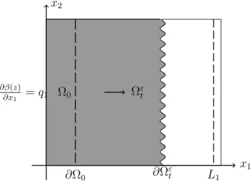
εtFigure 2.5: Neumann problem (6.1.1) in 2D case to estimate the value of r(q).
By the convergence in the Hausdorff distance, we see that T
ε→
L1r(q)−L0as ε → 0.
This allows us to estimate r(q) by choosing 0 < ε 1 and using
r(q) ≈ L
1− L
0T
ε.
We will find T
εnumerically by solving the problem on a bounded domain. To this end, we observe that if ε =
ω1for some ω ∈ N sufficiently large, the uniqueness of solutions of the ε-problem implies that Ω
ε, u
εare 1-periodic in the x
2-direction, that is, Ω
ε+ (e
2, 0) = Ω
ε, u
ε(x + e
2, t) = u
ε(x).
Therefore we introduce the numerical domain U = (0, 1)
2and solve the Hele-Shaw problem on U with boundary conditions
Ω
ε+ (e
2, 0) = Ω
ε,
u
x1(0, x
2, t) = q
10 ≤ x
2≤ 1, t ≥ 0, u(x
1, x
2+ 1, t) = u(x
1, x
2, t) x ∈ Ω
εt, t ≥ 0,
see Figure 2.5.
There are direct methods to solve the Hele-Shaw problem, however, for simplicity
and efficiency, we use the fact that the solution of the Hele-Shaw problem can be in the limit c → 0 approximated [12, 13] by the solution of the Stefan problem
cu
t− ∆u = 0 in Ω, V = g
ε|Du| on ∂Ω,
(2.3.1)
with initial condition u(·, 0) = u
0, where u
0is the 1-periodic-in-x
2solution of
−∆u
0= 0 in Ω
0\ K u
0= 0 on ∂ Ω
0,
∂
x2u
0= q
1on {x
2= 0}.
This problem can be rewritten in the enthalpy formulation by introducing β(s) :=
max(s, 0) and solving formally for z : R
n× R → R the solution of
cz
t− ∆β(z) = − ∂
∂t 1 g
εχ
int{z<0}in U × (0, ∞),
∂β(z)
∂x
1(0, x
2, t) = q
1x
2∈ [0, 1], t > 0, z 1-periodic in x
2,
z(·, 0) = u
0χ
Ω0− 1
cg
ε(·, 0) χ
Ω{0
in U,
(2.3.2)
where the first equation is understood in the sense of distributions. We can recover u as β(z) and Ω as {z > 0}.
If g
ε= g
ε(x), the well-posedness of problem (2.3.2) is well known from the theory of variational obstacle problems, see for example [14], [15], and u = β(z) is continuous [16]. We do not address the well-posedness when g
ε= g
ε(x, t), but show at least that (2.3.2) is equivalent to (2.3.1) with the same boundary data for classical solutions.
Let us therefore assume that there exists a differentiable function s : K
c→ [0, ∞),
Ds 6= 0 for t > 0, such that z ∈ C
2(Q
+) ∩ C
1(Q
+) ∩ C
1(Q
−) ∩ C(Q
−), z > 0 in Q
+, z(x, s(x)) = 0 if s(x) > 0, z < 0 in Q
−where
Q
±:= {(x, t) : x ∈ K
c, t > 0, ±(t − s(x)) > 0}.
By z ∈ C(Q
−) we understand the z has a limit denoted as z(x, s(x)−) as (y, t) → (x, s(x)) along sequences with t < s(y).
Assume that z satisfies (2.3.2), where the first equation is understood in the sense of distributions. Let us take a test function ϕ ∈ C
c∞(K
c× (0, ∞)). We have
0 = Z
Kc
Z
∞ 0czϕ
t+ β(z)∆ϕ − ∂
∂t 1 g
εχ
int{z<0}ϕ dx dt =
= Z
Q+
β(z)(cϕ
t+ ∆ϕ) dx dt + Z
Q−
czϕ
t− ∂
∂t 1 g
εϕ dx dt := I
++ I
−.
Integration by parts on the individual terms I
±yields
I
+= Z
Kc
Z
∞ s(x)cβ (z)ϕ
tdt dx + Z
∞0
Z
{s(x)<t}
β(z)∆ϕ dx dt
= − Z
Q+
(c∂
tβ(z) − ∆β(z))ϕ dx dt − Z
∞0
Z
{s(x)=t}
Dβ(z) · Ds
|Ds| ϕ dH
n−1dt where we used that z(x, s(x)) = 0 and that the unit outer normal vector to {x : s(x) < t} is
|Ds|Ds, and
I
−= Z
Q−
−cz
t− ∂
∂t 1 g
εϕ dx dt + Z
Kc
cz(x, s(x)−)ϕ(x, s(x)) dx.
From this we immediately have that u = β(z) satisfies cu
t− ∆u = 0 in Q
+, and z = −
cg1εin Q
−. In particular, z(x, s(x)−) = −
cgε(x,s(x))1. The coarea formula yields
Z
∞ 0Z
{s(x)=t}
Dβ(z) · Ds
|Ds| ϕ dH
n−1dt = Z
Kc
Dβ(z) · Dsϕ(x, s(x)) dx.
Therefore Z
Kc
− c
cg
ε(x, s(x)) − Du(x, s(x)) · Ds(x)
ϕ(x, s(x)) dx = 0.
But V =
|Ds|1and −Du · Ds = |Du||Ds| and therefore we conclude that
V = g
ε|Du|.
Stefan Problem
3.1 Stefan Problem
On the other hand, Stefan problem appeals Hele-shaw equation as the zero heat limit of One-phase Stefan problem. Mathematically they have almost the same equation structure, except in the heat operator. One-phase of Stefan problem itself describes a melting of ice with a region of water, where the temperature of the ice is preserved to be zero. The retained interests are to obtain the temperature in the water area and to understand the phase interface between ice and water.
Surely solving Stefan problem numerically in enthalpy form is more straightfor- ward than the temperature form. [17] implemented straightforward implicit finite difference to the enthalpy formulation of Stefan problem, and show the convergence of solution of the used modification Gauss-seidel method in order to solve a linear system.
In Stefan problem, refer to conservation law for energy, the change of heat amount per unit volume is u = ρc
PT where c
Pis the specific heat at constant pressure and T is a temperature. The heat flux has two components due to conduction
22
and transport. The flux from conduction is q = −k∇T where k denotes thermal conductivity. And the transport flux is ρc
PT V on the region of phase change.
Therefore the heat equation can be described by the following equation with assuming ρ, c
P, and k are constant.
∂T
∂t = k
ρc
P∆T , in the water area
∂T
∂t = 0 , in the ice area
∂T
∂t = ν
S· ∇T , on the phase change area.
(3.1.1)
Nevertheless, this work will consider the weaker form of (3.1.1) which physically describing the energy or more exactly enthalpy heat in the whole system. Given as the following equation for some parameter .
cu
t= ∆h(u) (3.1.2)
Where h(u) is defined as
h(u) = u
+(3.1.3)
represents the temperature.
We are interested in developing an efficient numerical method to find a free boundary decently and more importantly to adjust the solution of averaging velocity in a periodic media.
The weak formulation for Stefan problem is based on the extension of the equation
in term of temperature to the enthalpy energy balance, where the energy indicates
the absence of jump at the critical temperature due to the change of phase.
3.1.1 Enthalpy Formulation
Since the free boundary position is unknown and has to be determined each time t, numerically the solution of (SF1) cannot be obtained straightforward. Technically in the numeric point of view, it is simpler to consider the problem in the form of enthalpy energy equation instead than directly solving the equation (SF1).
Let u(·, ·) : R
n× {t > 0} → R . Physically u(x, t) can be describe the enthalpy per unit volume at position x and t. The enthalpy energy in the system consists of the heat energy and the work to change the physical state of the material. The enthalpy energy in the solid and liquid region can be written as
u(x, t) =
ρk
s(T (x, t) − T
melting) , T (x, t) < T
meltingin solid region ρk
l(T (x, t) − T
melting) + ρL , T (x, t) > T
meltingin the liquid region.
(3.1.4) where L is latent energy equals to −1/g in problem (SF1), k
sand k
lare respectively specific heat of solid and liquid. In one-phase case, when the temperature in solid state is preserved to be equal to T
melting= 0, we define β(·) : R 7−→ [0, ∞) is mapping the enthalpy to the temperature in one-phase ice and water region, such that β(u) = u
+. We realize that there exist a jump at critical temperature T
meltingdue to the change of phase caused by L, which in our case is not constant.
Thus, the enthalpy form of one-phase Stefan problem (with ρ = 1) is given by (SF2), where c = k
l.
cu
t− ∆β(u) = 0 in ( R
n\ K) × (0, ∞)
u = 1 in K × (0, ∞)
u(·, 0) = u
0in R
n(SF2)
3.1.2 Normal Velocity Derivation
Obviously since β is not even differentiable wherever u = 0, (SF2) can not give a point-wise interpretation to (SF1). Then, the equation can only be understood in the sense of distribution or weak sense. Formally we multiply (SF2) both side with test function ϕ(x, t) ∈ C
c∞(( R
n\ K) × (0, ∞)) and do integration by part. Let denote Q := ( R
n\ K ) × (0, ∞), then we do the following computation.
cu
t− ∆β(u) = 0 in Q
⇒ Z
Q
(cu
t− ∆β(u))ϕdxdt = 0 for any test function ϕ(x, t) ∈ C
c∞(Q)
⇒ 0 =c Z
Q
u
tϕdxdt − Z
Q
∆β(u)ϕdxdt
= − c Z
Q
uϕ
tdxdt + c Z
Rn\K
u(x, 0)ϕ(x, 0)dx +
Z
Q
∇β(u) · ∇ϕdxdt − Z
∂(Rn\K)×(0,∞)
∇β(u) · νϕdS (x)dt
= Z
Q
(−cuϕ
t+ ∇β(u) · ∇ϕ) dxdt
= Z
Q
(−cuϕ
t− β(u)∆ϕ) dxdt + Z
∂(Rn\K)×(0,∞)
β(u) ∂ϕ
∂ν dxdt
⇒0 = Z
Q
(cuϕ
t+ (βu)∆ϕ) dxdt
(3.1.5) Solution u of (3.1.5), is a weak solution (in distribution sense) of (SF2). And the equation (3.1.5) is called weak form of (SF2).
We denotes {u > 0} := (Ω
t\K)×(0, ∞) and {u < 0} := Ω
ct×(0, ∞). The area Q can
be split satisfying Q := {u > 0} ∪ {u < 0}, such that to be more specific we observe
the weak form in the following cases. We assume that u ∈ C({u > 0} ∪ {u < 0}),
β(·) ∈ C
2,1({u > 0}), and β(·) ∈ C
2,1({u < 0}).
For ϕ ∈ C
c∞({u > 0)}
0 = Z
Q
(cuϕ
t+ β(u)∆ϕ) dxdt
= Z
{u>0}
(cuϕ
t+ β(u)∆ϕ) dxdt
= Z
{u>0}
(−cu
tϕ − ∇β(u) · ∇ϕ) dxdt + Z
Ωt\K
cu(x, 0)ϕ(x, 0)dx +
Z
∂(Ωt\K)×(0,∞)
β(u) ∂ϕ
∂ν
xdSdt, (integration by part)
= Z
{u>0}
(−cu
tϕ − ∇β(u) · ∇ϕ) dxdt + 0
= Z
{u>0}
(−cu
tϕ + ∆β(u)ϕ) dxdt − Z
∂(Ωt\K)×(0,∞)
∇u · ν
xϕdSdt, (integration by part)
= Z
{u>0}
−(cu
t− ∆u)ϕdxdt + 0
⇒ cu
t− ∆u = 0
(3.1.6)
For ϕ ∈ C
c∞({u < 0}),
0 = Z
{u<0}
(cuϕ
t+ β(u)∆ϕ) dxdt
= Z
{u<0}
(cuϕ
t) dxdt, (since β(u) = 0 in {u < 0})
= Z
{u<0}
(−cu
tϕ) dxdt, by integration by part
⇒ cu
t= 0
(3.1.7)
Moreover, it is necessary to observe a weak form through the interface. In purpose
to obtain the formula for normal velocity on the interface, we assume the common
boundary of {u > 0} and {u < 0} is a smooth surface in R
n+1, and the complete
unit outer normal vector of {u > 0} denoted by ν = (ν
t, ν
x). So therefore we do
this following computation 0 =
Z
Q
(cuϕ
t+ β(u)∆ϕ) dxdt
= Z
Q
−cuϕ
t+ ∇β(u) · ∇ϕdxdt , ∀ϕ ∈ C
c∞(Q)
= Z
u>0
−cuϕ
t+ ∇β(u) · ∇ϕdxdt + Z
u<0
−cuϕ
t+ ∇β(u) · ∇ϕdxdt
= Z
u>0
(cu
t− ∆u)ϕdxdt + Z
∂{u>0}
(−cu, ∇u) · (ν
t, ν
x)ϕdS(x, t) +
Z
u<0
cu
tϕ − 0ϕdxdt + Z
∂{u<0}
(−cu, 0) · (−ν
t, −ν
x)ϕdS (x, t)
= Z
∂{u>0}
−cu|
+ν
t+ ∇u|
+· ν
x+ cu|
−ν
tϕdS (x, t)
(3.1.8)
Therefore, on the free boundary of {u > 0}, it is satisfied the following formula.
∇u|
+· ν
x+ cu|
−ν
t= 0 on ∂ {u > 0} (3.1.9)
Normal vector on the moving boundary.
(ν
t, ν
x) = 1
p (u
t|
+)
2+ |∇u|
+|
2(u
t|
+, ∇u|
+)
Therefore, the formula for the normal velocity can be written as follow.
0 = ∇u|
+· ν
x+ cu|
−ν
t= |∇u|
+|
2+ cu|
−u
+t⇒ u
+t|∇u|
+| = −|∇u|
+| cu|
−= 1
c g(x)|∇u|
(3.1.10)
Considering u from the negative side as, u|
−= −
gc1(x)= −
cg(x)1, we will obtain the
same formula of normal velocity as in Hele-Shaw equation (HS). Therefore, by
taking limit c → 0 the solution of Latent heat problem (SF2) in area {u > 0} is
expected to approach the given Hele-Shaw Problem, where {x ∈ R
n|(x, t) ∈ {u >
0}} was denoted as Ω
tin the Hele-Shaw equations.
It implies to the chosen of initial data u
0. Therefore if we expect to approximate HS by system (SF2), the initial data u
0require to be the following form,
u
0= 1
K+ 1
Ω0\Kv − 1
Ω0c1
g
c(3.1.11)
where Ω
0is a given initial domain, and v is harmonic function in Ω
0\ K.
Meanwhile, in one-phase Stefan problem such an ice melting, the problem is to find a function T (x, t) and free boundary ∂Ω
twhich satisfying:
cT
t− ∆T (x, t) = 0 for (x, t) ∈ (Ω
t\ K) × (0, ∞) T
t= g(x, t)|∇T |
2, for(x, t) ∈ ∂Ω
t× (0, ∞) T (x, t) = 1 for(x, t) ∈ K × (0, ∞)
T (x, t) = 0 for(x, t) ∈ ( R
n\ Ω
t) × (0, ∞) T (x, 0) = T
0(x) for x ∈ R
n(SF1)
The problem models the ice material contacting the water, which in one-phase case the ice temperature is preserved to be 0
◦C. The constant c represent a specific heat of water, and −1/g(x, t) represents the latent energy of ice with g > 0.
In [18], it discusses the asymptotic convergence of the SF to HS. It states for 1 dimensional case when g(x, t) is constant in x and t, the self-similar solution of u and T converge to the same constant as t → ∞ for every fixed x > 0, Yet the convergence is not uniform. Despite the free boundary of both problem have the same growth rate √
t, the free boundary of 1-D Stefan problem converge to
Hele-Shaw when c → 0.
Different to the 1-D case, problem SF is not ultimately to be HS as t → ∞, for n >= 2 there is only the convergence behavior to a stationary state of both problem, and the asymptotic behavior is different. Meanwhile, in 2-dimensional case, it shows that the SF simplifies to HS. Unlikely in the 1-D case, the HS and SF problem for multidimensional spaces do not always have a classical solution.
However, they always have a weak solution globally in time.
Explicit Methods and Implementation
4.1 Explicit Finite Difference Method
4.1.1 Discretization Scheme for One Dimensional Case
In this section we explain how to apply explicit finite difference to obtain numeric solution for u of (SF2). In the scheme, we implement the explicit form, so that the computation is restricted by the stability condition. In order to apply Finite Difference Method for numerical purpose, space domain in problem (SF2) restricted to be bounded, such that for 1-D case we consider problem (4.1.1).
cu
t− ∆β(u) = 0 in (0, X
max) × (0, ∞)
u = 1 in (−∞, 0] × (0, ∞)
β
x(u)(X
max, t) = 0 for t ∈ (0, ∞)
u(x, 0) = 1
(−∞,0]+ 1
(0,xf(0))v − 1
[xf(0),Xmax)g1c(4.1.1)
30
where v is a linear decrease monotone function in (1, x
f(0)) with v (0) = 1.
4.1.1.1 Numerical Scheme
Let M be a number of discretization points for domain of x such that for some X
maxsatisfying (0, x
f(t)) ⊂ [0, X
max), ∆x =
XMmax.
And u
kidenote a value of solution u in the discrete note (i∆x, k∆t). The discretized scheme for the equation cu
t= ∆β(u) can be written by standard Finite difference scheme as:
u
k+1i= u
ki+ ∆t
c∆x
2β(u
ki−1) − 2β(u
ki) + β(u
ki+1)
(4.1.2)
for k = 0, 1, · · · , N
Tand i = 1, 2, ·, M − 1 with stability condition,
∆t c∆x
2< 1
2 . (4.1.3)
4.1.1.2 Adjusting Free Boundary Position
In solving Hele-Shaw problem through the Stefan equation describe above, It is noteworthy to decently adjust the free boundary position in the problem. For one-dimension case we consider that numeric position of free boundary is computed as :
x
kf= min{x
i|u
kiu
ki+1< 0, i = 0, 1, ..., M − 1} (4.1.4) or by interpolation as described at figure 4.1, such that the free boundary position is approximated as formula (4.1.5).
x
kf≈ x ˆ
f= x
i+ ∆x( u
ki−1u
ki−1− u
ki− 1) (4.1.5)
∆x u
ki−1u
kix
i−1x
ix ˆ
fx
fx
i+1Figure 4.1: Extrapolation to estimate ¯ x
f4.1.2 The scheme for Two Dimensional Case
Let D ⊂ R
2be a bounded rectangle domain, and given closed set K ⊂ D. In order to apply finite difference method in 2-D case, we assume u always be differentiable on ∂D such that for numerical purpose, we consider problem (4.1.6),
cu
t− ∆β(u) = 0 in (D \ K) × (0, ∞) u(·, t) = 1 in K × (0, ∞)
∂β(u)
∂n
= 0 on ∂D × (0, ∞)
u(·, 0) = u
0in R
n(4.1.6)
where the initial condition u
0follows the form at (3.1.11).
4.1.2.1 Numerical Scheme
We assume that ∆y = ∆x. The discretization scheme of explicit method for (4.1.6) as follows.
u
k+1i,j= u
ki,j+
∆t c∆x
2{β(u
ki−1,j)
+ β(u
ki+1,j) − 4β(u
ki,j) + β(u
ki,j+1) + β(u
ki,j−1)}
(4.1.7)
with stability condition,
∆t c∆x
2< 1
4 . (4.1.8)
4.1.2.2 Adjusting Numeric Free Boundary in 2D Cartesian Grid
• • •
•
•
•
p
i,jp
i−1,jp
i+1,jp
i,j−1p
i,j+1u < 0
u > 0
u = 0
Figure 4.2: Boundary lies on the Cartesian grid between a 5-point stencil
Similarly to the scheme explained above. In order to adjust free boundary position lying on the Cartesian grid, we consider the situation of boundary across the grid between the 5-point stencil, where the center point as the reference. Figure 4.2 describes a situation when the boundary lies on the grid in 5-point stencil, where p
i,0is a reference point. Since in our case, the boundary represents ∂ {u > 0} where the solution of Hele-shaw defined, we consider P
i,0which returning u > 0 as the approximation of boundary position.
We may also extrapolate the position of free boundary crossing the legs of a 5-point stencil, by using two closest points in {u > 0} side straight through the edge.
4.2 Numerical Results and Discussion
4.2.1 One Dimensional Case
Let K = (−∞, 0], Ω
0= (−∞, x
f(0)) for given x
f(0), and K ⊂ Ω
0, and Ω
t=
(−∞, x
f(t)). The exact solution of 1-dimensional Hele-Shaw problem for the given
Ω
0and K is as follow.
u(x, t) =
1 , for (x, t) ∈ K × [0, ∞) 1 −
xxf(t)
, for (x, t) ∈ Ω
t\ K × [0, ∞), x
f(t) > 0 0 , for (x, t) ∈ Ω
tc× [0, ∞)
(4.2.1)
and the velocity at x
f(t) is given by:
V
n= x
0f(t) = g(x
f, t)|∇u(x
f, t)| = g(x
f, t)
x
f(t) , by taking constant g (x, t) = 1 (4.2.2) and noticing that x
f(t) is non-decreasing function with x
f(0) > 0, we obtain :
dx
f(t)
dt = 1
x
f(t)
⇒ x
f(t) = q
2t + x
f(0) is the solution of free boundary for this particular case.
4.2.1.1 Numerical Solution
To confirm the accuracy, we implement the scheme to the particular case and compare the result to its analytic solution.
0.0 0.2 0.4 0.6 0.8 1.0 1.2
t 1.0
1.2 1.4 1.6 1.8
xf(t)
exact num
0.0 0.2 0.4 0.6 0.8 1.0 1.2
t 0.004
0.005 0.006 0.007 0.008 0.009
|xk f
xf(t)|
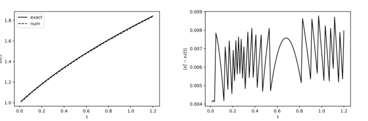
Figure 4.3: Free Boundary Position and its absolute error
Figure 4.3 shows the numerical solution of free boundary position in time from
Finite Difference Method (showing on the left), and its error computation, e =
|x
kf− x
f(k∆t)| (on the right). We can see from the error that the method is not satisfying enough, max
t|e| > ∆x for small enough = 10
−4. Figure 4.4 shows the error of numerical solution is still big enough. Nevertheless, it shows an error reduction in time.
0.0 0.2 0.4 0.6 0.8 1.0 1.2
t 0.0020
0.0025 0.0030 0.0035 0.0040 0.0045 0.0050 0.0055
|e|