Long‑time behavior of the one‑phase Stefan problem in periodic media and random media
著者 ブ ティ トゥ ザン
著者別表示 Vu Thi Thu Giang journal or
publication title
博士論文本文Full 学位授与番号 13301甲第4720号
学位名 博士(理学)
学位授与年月日 2018‑03‑22
URL http://hdl.handle.net/2297/00051435
Creative Commons : 表示 ‑ 非営利 ‑ 改変禁止
Dissertation
Long-time behavior of the one-phase Stefan problem in periodic media and
random media
Graduate School of
Natural Science & Technology Kanazawa University
Division of Mathematical and Physical Sciences
Student ID No.: 1524012007
Name: Vu Thi Thu Giang
Chief advisor: Prof. Seiro Omata
Date of Submission: March 8, 2018
Contents
Contents i
List of Figures iii
1 Introduction 1
1.1 Introduction . . . . 1 1.2 Notation . . . . 4 2 The one-phase Stefan problem and the Hele-Shaw problem 5 2.1 Mathematical modeling and classical formulation . . . . 5 2.2 Notion of solutions . . . 12 2.3 Homogenization and long-time behavior problems . . . 20 3 Long-time behavior of the one-phase Stefan problem in periodic
and random media 25
3.1 Preliminaries . . . 31 3.2 Uniform convergence of the rescaled variational solutions . . . 38 3.3 Uniform convergence of the rescaled viscosity solutions and free bound-
aries . . . 43 4 Long-time behavior of one-phase Stefan-type problems with anisotropic
diffusion in periodic media 52
4.1 Preliminaries . . . 58 4.2 Uniform convergence of the rescaled variational solutions . . . 70 4.3 Uniform convergence of the rescaled viscosity solutions and free bound-
aries . . . 79
A The fundamental solution of an uniformly elliptic equation of
divergence form 86
List of Figures
Figure 2.1 Semi-infinite slab melting from x = 0 due to a heat source h(t) at x = 0 . . . . 6 Figure 2.2 Hele-Shaw flow between two parallel flat plates separated by a
small gap of width h with the infinite pressure at the origin. . . . . 9 Figure 2.3 Singularities on the free boundary. (a)Two disc-shaped water
regions that move independently, (b)Merging of the two disc at a later
time. . . . 13
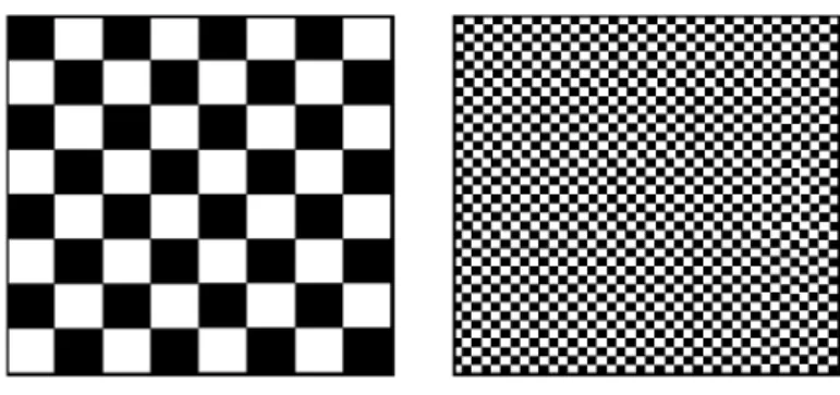
Figure 2.4 Checkerboard medium with self-averaging property . . . 21
Acknowledgement
First and foremost, I would like to express my sincere gratitude to my chief advisor, Professor Seiro Omata, for his constant support and guidance of my Ph.D. study.
He has been giving me all the best opportunities to study and gain the knowledge through the time of doing research. I also wish to thank my other advisor and mentor, Assistant Professor Norbert Poˇ z´ ar, for introducing me the topic of the one-phase Stefan problem as well as for his patience and encouragement in many invaluable discussions. I have the deepest respect and admiration for my both academic advisors.
I am also grateful to the Professors in Division of Mathematical and Physical Sciences, Graduate school of Natural Science and Technology, Kanazawa University, whose interesting lectures and talks that I had a chance to attend. I was especially impressed with the immense knowledge provided in the classes and seminars by Professor Masato Kimura and Professor Norihisa Ikoma. They all bring me a great academic environment and inspire me to the study of partial differential equations.
Besides, I would like to thank all members in my laboratory for their friendly help during the time we worked together. I especially want to thank Yoshiho Akagawa, whom I bothered with many problems not only in studying but also in dealing with the procedures in Kanazawa University.
Also many thanks to my teachers in Department of Mathematics and Informat- ics, Hanoi National University of Education, who taught me from the beginning to love mathematics with its own beauty despite many difficulties and challenges.
I have received financial support from Vietnamese Government through the Min- istry of Education and Training, VIED (Vietnam International Education Develop- ment) scholarship programs, project 911, for which I am very thankful.
I would like to acknowledge all my colleagues in Department of Mathematics,
Faculty of Information Technology, Vietnam National University of Agriculture who supported me with my job when I left for studying.
Our life in Kanazawa would be much more difficult without the precious help of many Vietnamese and Japanese friends, to whom I would like to send warm thanks.
Last but not least, I would like to deeply thank my family for their support and sacrifice. My parents unconditionally love and assist me, my husband and my sons constantly understand and take the time for me to do my research. This thesis is dedicated to my beloved sons, Nguyen Tri Khang and Nguyen Tri Kien, with the hope that it encourages them to study in the future.
Kanazawa, March 8, 2018
Chapter 1 Introduction
1.1 Introduction
The mathematical theory of partial differential equations (PDEs) has a long history motivated by various physical phenomena such as sound, heat, fluid dynamics, elas- ticity, quantum mechanics, etc. However, in many recent developments, PDEs find their practical applications in other fields of science as well like quantum chemistry, chemical kinetics, biology, economics and financial mathematics, or computer sci- ence. Some PDEs also come from the pure mathematical problems of other branches.
In a boundary-initial value problem, which is the classical subject in the theory of PDEs, the domain of the governing equation is fixed in space with specified data on the boundary and at the initial time. Such problems were well studied in both stan- dard analytical and numerical solution techniques. The more recent trend in PDEs is to consider free boundary problems or moving interface problems with totally dif- ferent features, namely, the space domains of the equations are separated by free boundaries which are neither fixed nor known a priori and need to be determined together with the solution.
Due to the difficulties from the unknown geometric information together with the
nonlinear nature and the singularities of the moving boundaries, only some simplest
free boundary problems have been showed to have classical solutions. It gave rise to
the question of generalizing the notion of solutions and defining some kinds of weak
solutions. The study of the regularity of the solution as well as the free boundary
itself, once the unique weak solution exists, is also one of the most interesting topics
in the field of free boundary problems. Beside the interests of the well-posedness of a PDE and the regularity of the solution, the homogenization problems for finding an average solution of equations with highly oscillating coefficients have received a lot of attention. Although the theory of homogenization was studied extensively for classical initial boundary value problems, there are still many open questions for homogenization of free boundary problems.
Among various types of free boundary problems, the Stefan problem is one of the most classical ones, which typically models the melting (the phase transition) of ice in contact with a water region due to heat conduction and an exchange of latent heat energy. This physical problem was formulated in a mathematical model by Slovene physicist and mathematician Josef Stefan (1835-1893) who treated the formation of ice in the polar seas (Stefan 1891), and was considered earlier by Lam´ e and Clapeyron (1831). The mathematical formulation of the problem consists of the heat equation in each phase, the solid and the liquid phase, and an additional condition at the free boundary, which is the so-called Stefan condition, that expresses the local velocity of a moving boundary. A very common simplification of the Stefan problem is the problem when we assume that the temperature is fixed at one of the phases (usually by assuming that the body of ice is maintained at temperature 0) and it is called the one-phase Stefan problem. The one-phase Stefan problem then contains only one heat equation in the liquid phase and a simpler form of the Stefan condition by eliminating one of the temperature gradients. The related Hele-Shaw problem is usually referred to in the literature as the quasi-stationary limit of the one-phase Stefan problem when the heat operator is replaced by the Laplace operator. This problem typically describes the flow of an injected viscous fluid between two parallel plates which form the so-called Hele-Shaw cell, or the flow in porous media.
The one-phase Stefan problem and Hele-Shaw problem in homogeneous media
in dimension n = 1 have the explicit classical solution ( [49]). However, we cannot
expect to have the classical solutions of both problems in dimension n ≥ 2 due to the
singularities on the free boundary which might develop in finite time. Thus there
are several approaches to define a notion of solutions including the notion of weak
solutions in the sense of distributions, the notion of variational inequalities solutions
and the notion of viscosity solutions. We will use the notion of weak solutions
based on the variational inequality formulation and the notion of viscosity solutions in our investigation. The well-posedness in a weak sense and regularity of these problems were studied in detail by many authors such as Friedman, Kinderlehrer, Rodrigues, Caffarelli, etc. (see [21, 51, 53, 7, 8, 34] and references therein). The problem is also well-posed in viscosity sense and the coincidence of two notions of solutions was obtained by Kim and Mellet [34, 38, 39]. Furthermore, the asymptotic behavior of solutions has gained some attentions in the literature. The asymptotic homogenization of the Hele-Shaw and the one-phase Stefan problem was given in [50, 38, 39]. The convergence of the Stefan problem to Hele-Shaw as t → ∞ in homogeneous media was observed in [49]. Moreover, the long-time behavior of the related Hele-Shaw problem was studied in detail in [45].
In our recent work, we focus on the long-time behavior of the one-phase Stefan and Stefan-type problems in some inhomogeneous media in dimension n ≥ 2. Using the technique of rescaling which is consistent with the evolution of the free boundary, we are able to show the homogenization of the free boundary velocity as well as the locally uniform convergence of the rescaled solution to a self-similar solution of the homogeneous Hele-Shaw problem with a point source for classical multi-dimensional one-phase Stefan problem. In the anisotropic case, when the heat operator is gener- alized by parabolic operators of divergence form, we also obtain the homogenization of the elliptic operator, where the rescaled solution now converges locally uniformly to a self-similar solution of the homogenized Hele-Shaw-type problem with a point source. Moreover, by viscosity solution methods, we furthermore deduce that the rescaled free boundary uniformly approaches that of the homogeneous Hele-Shaw problem with respect to the Hausdorff distance.
In this chapter, we state some notations for the convenient use later. In Chap-
ter 2, we present some basic background of our problem, which motivated us to
consider the long-time behavior of the solutions. In Chapter 3, we investigate the
asymptotic behavior of the isotropic inhomogeneous one-phase Stefan problem for
long times in periodic and random media. The main reference of Chapter 3 is a
joint-work of the author with N. Poˇ z´ ar [47]. The treatment of asymptotic long-
time behavior of anisotropic inhomogeneous Stefan-type problems is presented in
Chapter 4 with the main reference [48] which is another joint-work of the author
with N. Poˇ z´ ar. It turns out that when we replace our simple heat equation by
more general parabolic operators of divergence form, the construction of barriers is more challenging. Thus in this case, we restrict our consideration to the problems in dimension n ≥ 3 and in periodic media. Finally, Appendix A covers some basic techniques of the fundamental solution of a uniformly elliptic equation of divergence form used in our arguments.
1.2 Notation
We will use the following notations throughout this work.
For a set A, A
cis its complement.
Given a nonnegative function v, we denote the positive set and free boundary of v by
Ω(v) := {(x, t) : v(x, t) > 0}, Γ(v) := ∂ Ω(v), and for fixed time t,
Ω
t(v) := {x : v (x, t) > 0}, Γ
t(v) := ∂Ω
t(v).
(f)
+is the positive part of f : (f )
+= max(f, 0).
We will denote the general elliptic operator of divergence form and its rescaling as
Lu = D
i(a
ijD
ju), L
λu = D
i(a
ij(λ
1/nx)D
ju),
where we have used the Einstein’s summation convention.
Chapter 2
The one-phase Stefan problem and the Hele-Shaw problem
2.1 Mathematical modeling and classical formulation
2.1.1 The Stefan problem
As introduced above, the Stefan problem is a mathematical model, which typically describes the process of phase transitions, the melting or freezing, between solid (ice) and liquid (water) driven by the heat conduction and the exchange of latent heat. The problem has numerous applications in industry and technology such as the casting in manufacture of steel, the melting in thermal storage system, the evaporation of water, the drying of food, etc., see [1, 27, 58, 18, 59] . We begin with the most basic formulation of the Stefan problem to model the melting of a semi- infinite solid in contact with a liquid region containing a fixed source, for example a thin block of ice occupying the region 0 ≤ x < ∞ that melts due to the heating by a heat source at the fixed boundary x = 0 (see Fingure 2.1).
We assume that the temperature in the solid phase is a constant, say, the ice is maintained at temperature 0. At the fixed boundary, we prescribe a time dependent positive continuous boundary data h(t). The moving phase-change boundary is described by x = s(t). At time t, the liquid occupies the subset Ω(t) := {x : 0 < x <
s(t)} ⊂ [0, ∞) and the free boundary is Γ(t) := {x = s(t)}. As time t increases, Γ(t)
Figure 2.1: Semi-infinite slab melting from x = 0 due to a heat source h(t) at x = 0 .
travels from the left to the right and the liquid domain Ω(t) expands in the melting process. The classical formulation of this problem is the temperature distribution v(x, t) in the liquid phase and the location of the free boundary x = s(t). Even though there are two phases present, the problem is called a one-phase problem since the temperature is unknown only in the liquid phase.
1D Stefan problem. Find functions x = s(t) and v(x, t) : (0, ∞) × [0, ∞) → [0, ∞) satisfying
The liquid region 0 ≤ x < s(t)
ρcv
t= kv
xx, The heat equation in Ω(t) × (0, ∞), v(0, t) = h(t), The fixed boundary data, t > 0, v(x, 0) = 0, The initial data,
The free boundary x = s(t)
Lρs
0(t) = −kv
x(s(t), t), The Stefan condition,
s(0) = 0, The initial position of the interface, v(s(t), t) = 0, The continuity of temperature, The solid region, s(t) < x < ∞,
v(x, t) = 0, The solid is maintained at temperature 0 for all t > 0.
Here ρ is the density, c is the specific heat, k is the thermal conductivity of the
liquid and L is the latent heat. In the liquid region, the temperature is governed
by the standard heat diffusion. The Stefan condition is important to include the
phase change to the model and can be understood by the energy conservation law
as follows. Assume that the temperature depends only on the horizontal direction
and let A be a small portion of the interface at time t = t
0having area S. At time
t
0, the free boundary position is s(t
0). As the solid melts, at time t, the boundary
position is s(t) and the portion A has moved and formed a volume V . The energy we need to change the volume V of solid into liquid from time t
0to t is
E
1= LρV = LρS(s(t) − s(t
0)),
where L is the latent heat, the energy required to change one unit mass of substance from solid to liquid. On the other hand, the energy delivered through the portion A from time t
0to t can be computed as
E
2= Z
tt0
Z
A
q · ν
outdτ dS = S Z
tt0
q · ν
outdτ,
where q is the heat flux density and ν
out= (1, 0, 0) is the unit outward normal vector. By Fourier’s law of heat transfer, q = −kDv where k is a positive constant called the thermal conductivity of the liquid and D is the gradient. Then putting it in E
2we have
E
2= S Z
tt0
−kv
x(s(τ ), τ )dτ.
By the balance of energy, E
1must equal E
2. Divide both sides by (t − t
0) and take the limit as t tends to t
0. With the help of the mean value theorem we have
Lρs
0(t
0) = −kv
x(s(t
0), t
0).
The phenomenon of solidification is formulated similarly. This problem can model the phenomenon in two or three dimensional space where v is a function of two or three variables. The derivation of the Stefan condition on the interface is similar with noting that V = SV
νout(t −t
0), here V
νoutis the outward normal velocity, ν
outis the outward unit normal vector of the moving boundary and then we have
LρV
νout= −kDv · ν
outon {x = s(t)}.
Since the free boundary is a level set of v then ν
out= −
|Dv|Dvand V
νout=
|Dv|vtand we have an alternative form of the Stefan condition which is sometimes more useful for analytical treatment as
v
t= k
ρL |Dv|
2.
Without loss of generality, we can assume that the constants are 1.
The mathematical problem is naturally generalized to an arbitrary dimension
n ≥ 1 and is still called the one-phase Stefan problem. Thus, the one-phase Stefan
problem that we usually refer to is the following problem.
The multi-dimensional one-phase Stefan problem. Let n ≥ 1, K ⊂ R
nbe a compact set. The one-phase Stefan problem (on an exterior domain) is to find a function v(x, t) : R
n× [0, ∞) → [0, ∞) and a set {v > 0} satisfying
v
t− ∆v = 0 in {(x, t) : v(x, t) > 0, x ∈ R
n\K},
v = h on K,
v
t= |Dv|
2on ∂{v > 0}, v(x, 0) = v
0(x) on R
n,
(2.1)
where v
0and h = h(x, t) are given functions.
The one-phase Stefan problem can be generalized in many situations. First, if we assume that the temperature can vary in both phases, then we have the so- called two-phase Stefan problem. The derivation is analogous with an additional heat equation in the second phase and a little more complicated form of the Stefan condition. Since we only focus on the one-phase Stefan problem in our work, we will not introduce the two-phase problem and refer to [54, 53, 28] for more details.
Moreover, if we assume that the constants in the model are now some nonnegative smooth functions, we can have some more complex models. For example, if we take ρ = c = k = 1 and L = 1/g(x), where g(x) > 0, then we will have the Stefan condition of the form v
t= g(x)|Dv|
2. This problem is the one-phase Stefan problem with an inhomogeneous latent heat of phase transition, which is the subject for investigation of the next chapter. Furthermore, if in addition we assume that the heat diffuses in an anisotropic body, then the thermal conductivity coefficients vary through space and time, the heat flux vector q is expressed as q = −KDv, with matrix K = (k
ij(x, t)). Then the heat equation in the positive set becomes a more general parabolic equation of divergence form v
t− div(KDv) = 0 and the Stefan condition becomes v
t= g(x)KDv · Dv. In Chapter 4, we will deal with this type of the one-phase Stefan problem with some more assumptions on the coefficients, say, K is a symmetric, bounded, uniformly elliptic matrix, independent of time.
Finally, if we consider the problem with zero specific heat, i.e., c = 0 then the heat
operator simplifies into the Laplace operator and the problem is usually referred to
the (one-phase) Hele-Shaw problem, which will be introduced in the next section.
2.1.2 The Hele-Shaw problem as the quasi-stationary limit of the Stefan problem
The classical Hele-Shaw problem is a two-dimensional mathematical model that typically describes the flow of an injected viscous fluid in the thin gap between two parallel plates, see Fig.2.2.
Figure 2.2: Hele-Shaw flow between two parallel flat plates separated by a small gap of width h with the infinite pressure at the origin.
The governing equations of this problem are derived by gap-averaging the three- dimensional Navier-Stokes equations as in [40, 29]. We will sketch some of main features of this problem here. Let us consider the flow of a Newtonian, incom- pressible, inviscid fluid, driven by the singularity of a point source at the origin.
Assume that at time t, the fluid occupies a domain Ω(t) in the (x, y)-plane with free boundary Γ(t) := ∂Ω(t). If the injected fluid is slow enough for the flow to be approximately stationary and the gap between two parallel plates h is small enough, following [40, 29], the averaged velocity over the gap v :=
h1R
h0
vdz satisfies v = − h
212µ Dp in Ω(t) (2.2)
away from singularity, where p is the pressure of the fluid, h is the distance be-
tween two plates and µ is the dynamic viscosity of the fluid. Moreover, by the
incompressibility of the flow, div v = 0 and thus we have
∆p = 0 in Ω(t)\{0}.
We also need to specify the boundary condition on the moving interface Γ(t). If we neglect the surface tension effects, the dynamic boundary condition is given by
p = 0 on Γ(t).
The kinematic boundary condition states that the fluid particles on the interface remain on the interface for all time by the condition
V
νout= v · ν
outon Γ(t),
where ν
outis the unit outward normal vector on Γ(t). By (2.2), on Γ(t), V
νoutcan be written as
V
νout= −kDp · ν
out, (2.3)
where k =
12µh2. Similar to the Stefan condition formulation, since the free boundary is a level set of p, (2.3) can also be expressed as p
t= k|Dp|
2. This problem is usually generalized to an arbitrary dimension. If k is a constant then we have a homogeneous problem. We also have a flow in an inhomogeneous medium when k is given by a function and in this case, we will have a finger shape interface as in Figure 2.2. In our work, the limit problem is the homogeneous the Hele-Shaw problem with a point source formally given as follows.
The multi-dimensional Hele-Shaw problem with a point source. Let n ≥ 1, the Hele-Shaw problem with a point source is to find a function p(x, t) : R
n× [0, ∞) → [0, ∞) and a set {p > 0} satisfying the free boundary problem
∆p = 0 in {p > 0}, p
t= |Dp|
2on ∂{p > 0}, p(x, 0) = 0 on R
n, lim
|x|→0
p Φ = C,
(2.4)
where Φ is the fundamental solution of the Laplace equation and C is a constant.
From the mathematical point of view, the Hele-Shaw problem can be regarded as
the one-phase Stefan problem when the interface moves slowly, the flow is approxi-
mately stationary and the specific heat c is negligible. Indeed, if in the Hele-Shaw
model, instead of the point source, we consider the movement under a fixed source K with a prescribed boundary data h(t) and assume that at the initial time, the pressure is given by some function p
0then we recover the following one-phase Ste- fan problem with zero specific heat if the pressure p of the fluid is regarded as the temperature of the liquid:
∆p = 0 in {p > 0}\K,
p = h on K,
p
t= |Dp|
2on ∂{p > 0}, p(x, 0) = p
0on R
n,
(2.5)
where p
0and h = h(t) are given functions. This problem is also called a Hele- Shaw-type problem. In some cases, the temperature and the free boundary in the one-phase Stefan problem depend continuously on c. Thus, the free boundary of the Stefan problem approaches that of the Hele-Shaw problem as c → 0. Moreover, as t → ∞ the diffusion in the process usually reaches the steady-state and the heat equation in the Stefan problem loses the first term v
t. Thus, we also expect to get the coincidence between the solutions as well as the free boundaries of these two models in the asymptotic limit when t → ∞.
The asymptotic convergence of the Stefan problem to Hele-Shaw is indeed the consideration in [49], where the authors analyzed the asymptotic behavior of weak solutions of both models in the multi-dimensional case n ≥ 2. They explained the asymptotic behavior of the solutions in term of the near-field limit, i.e., the limit of the solutions at a fixed point x in the space as time t → ∞, and the far-field limit, i.e., the development in the region close to the free boundary. In the near-field limit setting, the results in [49] stated that in both cases, the solutions converge to the solution of the Dirichlet exterior problem for the Laplacian while in the far-field limit, they converge to the solution of the Hele-Shaw problem with a point source.
The authors also showed that the free boundaries approach a sphere as t → ∞ with a precise asymptotic growth rate. The subjects of the study in [49] are the classical Stefan problem and Hele-Shaw problem in homogeneous isotropic media.
Their results give rise to the question: Do the results hold for the inhomogeneous anisotropic case?
The conclusions for the near-field limit can be automatically extended for the in-
homogeneous case and also for the anisotropic case with some simple modifications.
However, the developments for the far-field limit will be more complicated, since in [49] the analysis of the far-field limit is based on an appropriate rescaling and in an inhomogeneous setting, the homogenization problems for the free boundary velocity and the elliptic operator appear in the scaling limit. This question is par- tially answered by Poˇ z´ ar in [45] where the author proved that in an inhomogeneous medium, the rescaled solution of the Hele-Shaw problem locally uniformly converges to the solution of a homogeneous Hele-Shaw problem with a point source and the free boundary also converges to a sphere with respect to the Hausdorff distance. We will extend this result to the Stefan problem with an inhomogeneous latent heat in Chapter 3 and that with an inhomogeneous latent heat and anisotropic conductivity in Chapter 4.
In the Section 2.3 below, we will give a brief introduction of a homogenization problem and how it is related to our investigation. Before that we will recall some notions of solutions of the one-phase Stefan problem used in our work.
2.2 Notion of solutions
In this section, we will recall some notions of solutions of the one-phase Stefan problem (2.1) for the space dimension n ≥ 2. We consider the problem (2.1) with the initial data v
0satisfying
v
0∈ C
2(Ω
0\K ), v
0> 0 in Ω
0, v
0= 0, on Ω
c0:= R
n\ Ω
0, and v
0= 1 on K,
|Dv
0| 6= 0 on ∂Ω
0, for some bounded domain Ω
0⊃ K.
(2.6)
2.2.1 Classical solutions
Let G(t) := Ω
t(v) × {t} and Q
T:= S
0<t<T
G(t).
Definition 2.1. A classical solution of the one-phase Stefan problem in [0, T ] is a pair (v(x, t), Γ(t)) with v ∈ C(Q
T) T
C
2,1(Q
T), Dv ∈ C(Q
T\G(0))) and Γ(t) ∈ C
1((0, T ]) ∩ C([0, T ]) that satisfy (2.1).
In case the space dimension is n = 1, the existence and uniqueness of the classical
solution of the Stefan problem with monotone free boundary exits globally in time
for various kinds of boundary and initial data, see [19, 54]. However, the situation in
multi-dimensional space is much more complicated. As observed in [28, 20, 31], the singularities of the free boundary might develop in finite time such as the merging of water regions that move independently or the closing of an ice region to a point, or a piece of ice on melting, may break into two, etc. Thus, we do not expect that the classical solution exists for all time, even if the data are smooth. Nevertheless, the short time existence of the classical solution of (2.1) was established by Hanzawa in [30] for some sufficiently smooth compatible boundary and initial data.
Figure 2.3: Singularities on the free boundary. (a)Two disc-shaped water regions that move independently, (b)Merging of the two disc at a later time.
The lack of classical solutions of the one-phase Stefan problem motivated to the study of weak solutions. In our work, we will use the following notions of weak solutions and viscosity solutions.
2.2.2 Weak solutions
In 1981, Elliot and Janovsk´ y introduced a notion of weak solution to the Hele-Shaw problem by taking integration in time of the classical solution and transforming the problem into an elliptic variational inequality. Following this approach, it was observed later by Duvaut [14] that we also can formulate the one-phase Stefan problem as a parabolic variational inequality. This method was then developed by Friedman and Kinderlehrer [21], Caffarelli [7, 8] and many other authors.
To motivate this method, let us suppose that (v(x, t), Γ(t)) is a classical solution of the Stefan problem (2.1) and introduce u(x, t) := R
t0
v(x, s)ds. Fix R, T > 0 and
set B = B
R(0), D = B \K . Following [21], it can be shown that, if R is large enough
(depending on T ), then the function u solves a variational problem. Indeed, since
the free boundary Γ(t) is C
1((0, T ]) and v
t> 0 on Γ(t), we represent the positive
domain Ω(t) by Ω(t) = {x : s(x) < t} for some nonnegative function s such that Ω
0:= {x : v
0(x) > 0} = {x : s(x) = 0} . From the definition of u we have if x ∈ Ω
c0then s(x) > 0 and
u(x, t) =
0 if 0 ≤ t ≤ s(x),
Z
t s(x)v(x, s)ds if s(x) < t ≤ T.
Now direct computation gives u
xi=
Z
t s(x)v
xi(x, s)ds − s
xiv(x, s(x)) = Z
ts(x)
v
xi(x, s)ds, u
xixi=
Z
t s(x)v
xixi(x, s)ds − s
xiv
xi(x, s(x))
(2.7)
for x ∈ Ω
c0, t > s(x).
Since v satisfies (2.1) in classical sense then V
νout= |Dv|. On the other hand, since the positive domain of v is represented by s(x) then V
νout=
|Ds|1and therefore
|Dv||Ds| = 1, the vectors Dv and Ds are parallel (and parallel to ν
out) but in opposite directions then we have Dv · Ds = −1. In view of (2.1) and (2.7) we have
∆u(x, t) = Z
ts(x)
v
s(x, s)ds + 1
= v(x, t) + 1
= u
t(x, t) + 1.
Similarly, if x ∈ Ω
0then for all 0 < t ≤ T , u(x, t) = R
t0
v(x, s)ds, s(x) = 0 and
∆u(x, t) = Z
t0
v
s(x, s)ds
= v(x, t) − v (x, 0)
= u
t(x, t) − v
0(x).
Define
f(x) :=
v
0(x) if x ∈ Ω
0,
− 1 if x ∈ Ω
c0. Then finally u satisfies the nonlinear parabolic problem
u > 0,
(u
t− ∆u)(ϕ − u) = f (ϕ − u),
for any ϕ ∈ K(t), x ∈ D, s(x) < t < T
and
u = 0,
(u
t− ∆u)(ϕ − u) = 0 ≥ − ϕ = f (ϕ − u), ]
for any ϕ ∈ K(t), x ∈ D, 0 < t < s(x).
Here we set K(t) = {ϕ ∈ H
1(D), ϕ ≥ 0, ϕ = 0 on ∂B, ϕ = t on K }. We use the standard notation for Sobolev spaces H
k, W
k,p.
In conclusion, we have transformed the classical problem (2.1) into the following variational inequality problem.
Variational inequality problem. Find u ∈ L
2(0, T ; H
2(D)) such that u
t∈ L
2(0, T ; L
2(D)) and
u(·, t) ∈ K(t), 0 < t < T,
(u
t− ∆u)(ϕ − u) ≥ f(ϕ − u), a.e.(x, t) ∈ B × (0, T ) for any ϕ ∈ K(t), u(x, 0) = 0 in D.
(2.8)
Note that u(x, t) is independent of the choice of B as long as R is large enough [39, Lemma 3.6]. If v is a classical solution of (2.1) then u is a solution of (2.8), but the inverse statement is not valid in general. However, we have the following result [21, 51].
Theorem 2.2 (Existence and uniqueness of the variational problem). If v
0satisfies (2.6), then the problem (2.8) has a unique solution satisfying
u ∈ L
∞(0, T ; W
2,p(D)), 1 ≤ p ≤ ∞, u
t∈ L
∞(D × (0, T )),
and
u
t− ∆u ≥ f, u ≥ 0, u(u
t− ∆u − f ) = 0
a.e. in D × (0, ∞).
We will thus say that if u is a solution of (2.8), then u
tis a weak solution of the corresponding Stefan problem (2.1). The theory of variational inequalities for an obstacle problem is well developed, for more details, we refer to [21, 51, 38]. We now collect some useful results on the weak solutions from [21, 51].
Proposition 2.3. The unique solution u of (2.8) satisfies
0 ≤ u
t≤ C a.e.D × (0, T ),
where C is a constant depending on f. In particular, u is Lipschitz with respect to t and u is C
α(D) with respect to x for all α ∈ (0, 1). Furthermore, if 0 ≤ t < s ≤ T , then u(·, t) < u(·, s) in Ω
s(u) and also Ω
0⊂ Ω
t(u) ⊂ Ω
s(u).
Lemma 2.4 (Comparison principle for weak solutions). Suppose that f ≤ f. Let ˆ u, u ˆ be solutions of (2.8) for respective f, f ˆ . Then u ≤ u, ˆ moreover,
θ ≡ ∂u
∂t ≤ ∂ u ˆ
∂t ≡ θ. ˆ
Remark 2.5. Regularity of θ and its free boundary has been studied quite extensively, including Caffarelli and Friedman (see [7, 8, 22]). It is known that a weak solution is classical as long as Γ
t(u) has no singularity. The smoothness criterion (see [7, 22], [49, Proposition 2.4]) immediately leads to the following corollary.
Corollary 2.6. Radially symmetric weak solutions of the Stefan problem (2.1) are smooth classical solutions.
Remark 2.7. If we consider the problem with an inhomogeneous latent of phase transition L = 1/g(x) and an anisotropic diffusion K = (k
ij), then as shown in Section 2.1.1, the governing equation is a parabolic equation of divergence form
v
t− D
i(k
ijD
jv) = 0
in the positive domain and Stefan condition on the free boundary is given by v
t|Dv| = gk
ijD
jvν
i.
Here D is the space gradient, D
iis the partial derivative with respect to x
i, v
tis the partial derivative of v with respect to time variable t and ν = ν(x, t) is inward spatial unit normal vector of ∂{v > 0} at point (x, t) and we use the Einstein summation convention.
We can define a weak solution of this problem similarly to the homogeneous isotropic case. We only need to replace the heat operator by a more general parabolic operator of divergence form D
i(k
ijD
j) and change the form of f as
f (x) :=
v
0(x) if x ∈ Ω
0− 1
g (x) if x ∈ Ω
c0.
All computations and almost all results remain to be valid. There are only some issues concerning the regularity of θ in the anisotropic case. Furthermore, we do not have classical radially symmetric solutions in the anisotropic case, which will lead to some difficulties in constructing barriers for our arguments.
2.2.3 Viscosity solutions
The second notion of solutions we will use are the viscosity solutions introduced in [34]. The main results in this work include the well-posedness of the Stefan problem (2.1) and a comparison principle for viscosity solutions. We will recall here some important ideas of viscosity solutions taken from [34, 39].
First, for any nonnegative function w(x, t) we define:
w
?(x, t) := lim inf
(y,s)→(x,t)
w(y, s), w
?(x, t) := lim sup
(y,s)→(x,t)
w(y, s).
We will consider solutions in the space-time cylinder Q := ( R
n\K) × [0, ∞).
Definition 2.8. A nonnegative upper semicontinuous function v(x, t) defined in Q is a viscosity subsolution of (2.1) if the following hold:
a) For all T ∈ (0, ∞), the set Ω(v) ∩ {t ≤ T } ∩ Q is bounded.
b) For every φ ∈ C
x,t2,1(Q) such that v − φ has a local maximum in Ω(v) ∩ {t ≤ t
0} ∩ Q at (x
0, t
0), the following holds:
i) If v (x
0, t
0) > 0, then (φ
t− ∆φ)(x
0, t
0) ≤ 0.
ii) If (x
0, t
0) ∈ Γ(v), |Dφ(x
0, t
0)| 6= 0 and (φ
t− ∆φ)(x
0, t
0) > 0, then
(φ
t− g(x
0)|Dφ|
2)(x
0, t
0) ≤ 0. (2.9) Definition 2.9. A nonnegative lower semicontinuous function v (x, t) defined in Q is a viscosity supersolution of (2.1) if for every φ ∈ C
x,t2,1(Q) such that v − φ has a local minimum in Ω(v) ∩ {t ≤ t
0} ∩ Q at (x
0, t
0), the following holds:
a) If v(x
0, t
0) > 0, then (φ
t− ∆φ)(x
0, t
0) ≥ 0.
b) If (x
0, t
0) ∈ Γ(v), |Dφ(x
0, t
0)| 6= 0 and (φ
t− ∆φ)(x
0, t
0) < 0, then
(φ
t− g (x
0)|Dφ|
2)(x
0, t
0) ≥ 0. (2.10)
Now let v
0be a given initial condition with support Ω
0and free boundary Γ
0= ∂Ω
0, we can define viscosity subsolution and supersolution of (2.1) with cor- responding initial data and boundary data.
Definition 2.10. A viscosity subsolution of (2.1) in Q is a viscosity subsolution of (2.1) in Q with initial data v
0and boundary data 1 if:
a) v is upper semicontinuous in ¯ Q, v = v
0at t = 0 and v ≤ 1 on Γ, b) Ω(v) ∩ {t = 0} = {x : v
0(x) > 0}.
Definition 2.11. A viscosity supersolution of (2.1) in Q is a viscosity supersolution of (2.1) in Q with initial data v
0and boundary data 1 if v is lower semicontinuous in ¯ Q, v = v
0at t = 0 and v ≥ 1 on Γ,
And finally we can define viscosity solutions.
Definition 2.12. The function v(x, t) is a viscosity solution of (2.1) in Q (with initial data v
0and boundary data 1) if v is a viscosity supersolution and v
?is a viscosity subsolution of (2.1) in Q (with initial data v
0and boundary data 1).
Remark 2.13. By a standard argument, if v is the classical solution of (2.1) then it is a viscosity solution of that problem in Q with initial data v
0and boundary data 1.
The existence and uniqueness of a viscosity solution as well as its properties were studied in great detail in [34]. One important feature of viscosity solutions is that they satisfy a comparison principle for strictly separated initial data.
Definition 2.14. We say that a pair of functions u
0, v
0: D → [0, ∞) are (strictly) separated and denote by u
0≺ v
0in D ⊂ R
nif:
a) {u
0> 0} ∩ D is compact and b) u
0(x) < v
0(x) in {u
0> 0} ∩ D
Theorem 2.15 (Comparison principle, [34, 39]). Let v
1, v
2be respectively viscosity
subsolution and supersolution of (2.1) in Q. If v
1≺ v
2on the parabolic boundary
of Q, then v
1(·, t) ≺ v
2(·, t) in Q.
One of the main tool we will use in this work is the following Theorem about coincidence of weak and viscosity solutions. Following [39] we can state that:
Theorem 2.16 (Theorem 3.1, [39]). Assume that v
0satisfies (2.6). Let u(x, t) be the unique solution of (2.8) in B × [0, T ] and let v(x, t) be the solution of
v
t− ∆v = 0 in Ω(u)\K,
v = 0 on Γ(u),
v = 1 in K,
v(x, 0) = v
0(x).
(2.11)
Then the following hold:
a) v(x, t) is a viscosity solution of (2.1) in B × [0, T ] with initial data v(x, 0) = v
0(x).
b) u(x, t) = R
t0
v(x, s)ds
Proof. See proof of Theorem 3.1, [39].
Remark 2.17. We want to clarify the definition of a solution v when Ω(u) is not smooth. Since u is continuous and Ω(u) is bounded at all times (Lemma 3.6, [39]) then the existence of solution of (2.11) is provided by Perron’s method as follows:
v = sup{w|w
t− ∆w ≤ 0 in Ω(u), w ≤ 0 on Γ(u), w ≤ 1 in K, w(x, 0) ≤ v
0(x)}.
It may happen that v is not continuous through its boundary in general. However, from the regularity results of Caffarelli and Friedman, we know that in our case u
tis continuous in space and time, and we would have v = u
t.
The coincidence of weak and viscosity solutions gives us a more general compar- ison principle:
Lemma 2.18 (Corollary 3.12, [39]). Let v
1and v
2be, respectively, a viscosity sub-
solution and super solution of the Stefan problem (2.1) with continuous initial data
v
10≤ v
02and boundary data 1. In addition, suppose that v
01(or v
20) satisfies condition
(2.6). Then v
1?≤ v
2and v
1≤ (v
2)
?in R
n\K × [0, ∞).
Remark 2.19. Similar to the notion of weak solutions, we can define a viscosity solution of the one-phase Stefan problem with an inhomogeneous latent heat L =
1
g(x)
and an anisotropic conductivity K = (k
ij) as in Remark 2.7. For this problem, the definition of a viscosity subsolution (resp. a viscosity supersolution) is analogous to Definition 2.8 (resp. Definition 2.9), when we replace the Laplace operator by D
i(k
ijD
j) and (2.9) (resp. (2.10)) by
(φ
t− ga
ijD
jφν
i|Dφ|)(x
0, t
0) ≤ 0,
(resp. the inequality ≥), where ν is inward spatial unit normal vector of ∂ {v > 0}.
All the other definitions and results follow the same as in the homogeneous isotropic case.
2.3 Homogenization and long-time behavior problems
Homogenization theory is the study of partial differential equations with rapidly os- cillating coefficients and extract homogenized equations. Many problems in physics, mechanics or chemistry are processes in inhomogeneous media with a fine micro- scopic structure. For example, we consider the steady state of the heat flow in a periodic anisotropic medium which can be modeled by an elliptic equation of divergence form
div(A(x)Du(x)) = f (x) in Ω,
where Ω is an bounded domain in R
n, A(x) is a nonnegative, bounded, periodic matrix with period 1 and f is a smooth function. Now we look at the process from far away, the period of the medium will be much smaller than the length scale of Ω, say, period ε, we will then be concerned with the equation with rapidly oscillating coefficients
div A x
ε
Du
ε(x)
= f (x) in Ω.
When the scale of the microscopic periodic structure is very small in comparison
with the scale of the domain under consideration, the medium has homogenized (or
macroscopic) characteristics, see Figure 2.4 below.
Figure 2.4: Checkerboard medium with self-averaging property
Thus we expect that as ε → 0, u
ε→ u
0in an appropriate sense and u
0is a solution of a homogenized (or effective) equation
div A
0Du
0= f in Ω,
where A
0is a homogenized matrix with constant coefficients. The main concerns of the homogenization theory is to obtain the convergence (usually in a weak sense) of the solution u
εto u
0and to construct the homogenized matrix A
0(A
0is a constant matrix in many cases). The homogenization was first developed for periodic struc- tures and then generalized for other media with self averaging properties (almost periodic, stationary ergodic). The operator type in a homogenization problem also can be more general, time independent or dependent, linear or nonlinear. We would like to refer to [6, 32, 11, 12, 13, 57, 7, 8] for more details.
The homogenization problems appear in our investigation as the following ob- servation. Using the ideas in [49, 45], we will analyze the asymptotic behavior of the solution of the one-phase Stefan problem (2.1) in far region and large time by using an appropriate rescaling, i.e.,
v
λ(x, t) := λ
(n−2)/nv(λ
1/nx, λt) if n ≥ 3, and the corresponding rescaling for variational solutions
u
λ(x, t) := λ
−2/nu(λ
1/n, λt) if n ≥ 3
(see Section 3.1.1 for n = 2). It is a natural rescaling since as shown in [49],
the position of the free boundary expands with the rate |x| ∼ t
1/n. The rescaling
can be intuitively understood as looking at the solution from far away and for a
very long time. The difference between our setting and that in [49] is that instead of considering L to be a constant, we study the one-phase Stefan problem with an inhomogeneous latent heat L(x) =
g(x)1. Then the rescaled viscosity solution satisfies the free boundary velocity law
V
νλout= g(λ
1/nx)|Dv
λ|.
Let us assume that the latent heat of phase transition L(x) = 1/g(x) has averaging property, then it will average out as λ → ∞ and the velocity become homogenized as
V
νout= 1
h1/gi |Dv|,
where h1/gi represents the “average” of 1/g. The convergence process of the rescaled normal velocity to a limit with a homogeneous coefficient is a homogenization of the free boundary velocity. Moreover, if the Laplace operator is replaced by a periodic elliptic operator of divergence form L, then we see that v
λsatisfies
λ
(2−n)/nv
tλ− L
λv
λ= 0 in Ω(v
λ)\K
λ,
V
νλout= g(λ
1/nx)a
ij(λ
1/nx)D
jv
λν
ion Γ(v
λ),
where L, L
λwere defined in Section 1.2 and ν
out, ν are the outward and inward unit normal vector on Γ(v
λ) respectively. As λ → ∞, the parabolic operator becomes elliptic and the homogenization of the elliptic operator is also expected beside the homogenization of the free boundary normal velocity.
The rescaling for the variational solution is similar, the rescaled variational so- lution satisfies a variational inequality
(λ
2−nnu
λt− L
λu
λ)(ϕ − u
λ) ≥ f
λ(x)(ϕ − u
λ) (2.12) a.e. (x, t) ∈ R
n× (0, ∞), for any ϕ ∈ K
λ(t), where
f
λ(x) := f (λ
1/nx) =
v
0(λ
1/nx) if x ∈ Ω
λ0,
− 1/g(λ
1/nx) if x ∈ (Ω
λ0)
c,
Ω
λ0= Ω
0/λ
1/nand K
λ(t) = {ϕ ∈ H
1( R
n), ϕ ≥ 0, ϕ = λ
n−2nt on K
λ}. As λ → ∞,
we also expect to have the homogenization of the variational inequality and the
elliptic asymptotic convergence of the rescaled parabolic operator. Therefore, the
homogenization processes are in particular extremely important to our problem.
Even though the homogenization has a long history, most of the results were obtained for boundary value problems (or initial boundary value problems) in a bounded domain. There are very few results for the homogenization of a free bound- ary problem. Fortunately, the homogenization of the one-phase Stefan problem was studied by Rodrigues [50] for a periodic setting and generalized for a stationary er- godic setting by Kim and Mellet [39]. Kim and Mellet also obtained similar results for the Hele-Shaw problem earlier in [38]. However, our situation is considerably different when the domain of rescaled variational solution u
λchanges as λ → ∞. In fact, due to the rescaling, the fixed domain K shrinks to the origin and the solution gets singularity in the limit. Thus we need to characterize the singularity of solution as |x| → 0. For the isotropic inhomogeneous case in Chapter 3, this task can be done by following directly the barrier arguments in [45] for the Hele-Shaw problem.
In anisotropic inhomogeneous case of Chapter 4, since we cannot use the classical radially symmetric solution as barriers, we will construct some ones to modify the treatment in Chapter 3. Moreover, in the anisotropic case, we need to deal with the homogenization problem of the elliptic operator in the domain which together with the specified boundary data, change as λ varies. Therefore, the known results on the homogenization of the one-phase Stefan problem cannot be applied directly.
We will solve this problem with the help of the Γ-convergence techniques, which are classical approaches for homogenization of nonlinear variational problems, with some adaptations for our problem. Another characteristic of our problem which is significantly different with the previous work is the fact that we need to combine the homogenization problems with the long-time behavior problem. This kind of work was done for the Hele-Shaw problem in [45], however, the arguments in [45]
rely on the very useful monotonicity of solutions while we do not have this property in the Stefan problem. We will instead use a weaker monotonicity stated later. In addition, the rescaled parabolic equation becomes elliptic when λ → ∞, which also causes some issues in analyzing the convergence of the rescaled free boundary to the free boundary of the homogenized limit equation.
In our work, we will assume that the medium in the one-phase Stefan problem
is periodic or stationary ergodic over a probability space (A, F, P ). We recall [10,
38, 39] that a random variable g(x, ·) : A → R is said to be stationary ergodic if it
satisfies the following two conditions:
1. The distribution of the random variable g(x, ·) is independent of x (this prop- erty is referred as stationary). This can be expressed more precisely by the existence, for each x ∈ R
n, of a measure-preserving transformation τ
x: A → A such that:
g(x + x
0, ω) = g(x, τ
x0ω) for all x
0∈ R
nand ω ∈ A.
2. The underlying transformation τ
xis ergodic, that is, if B ⊂ A and τ
xB = B for all x ∈ R
n, then P (B) = 0 or P (B ) = 1.
This probabilistic setting, we can think about a random checkerboard for instance, is a general extension of the notions of periodicity for a function to have some self-averaging behavior. In particular, we will make use of the following important application of the subadditive ergodic theorem.(see [38, Lemma 4.1])
Lemma 2.20 (cf. [38, Section 4, Lemma 7], see also [45]). For given g satisfying (2), there exists a constant, denoted by h1/gi, such that if Ω ⊂ R
nis a bounded measurable set and if {u
ε}
ε>0⊂ L
2(Ω) is a family of functions such that u
ε→ u strongly in L
2(Ω) as ε → 0, then
ε→0
lim Z
Ω
1
g(x/ε, ω) u
ε(x)dx = Z
Ω
1 g
u(x)dx a.e. ω ∈ A.
Chapter 3
Long-time behavior of the one-phase Stefan problem in periodic and random media
We consider the one-phase Stefan problem in periodic and random media in a dimen- sion n ≥ 2. The aim of this chapter is to understand the behavior of the solutions and their free boundaries when time t → ∞. The contents of this chapter is based on the work that previously appeared in [47].
Let K ⊂ R
nbe a compact set with sufficiently regular boundary, for instance
∂K ∈ C
1,1, and assume that 0 ∈ int K. The one-phase Stefan problem (on an exterior domain) with inhomogeneous latent heat of phase transition is to find a function v(x, t) : R
n× [0, ∞) → [0, ∞) that satisfies the free boundary problem
v
t− ∆v = 0 in {v > 0}\K,
v = 1 on K,
V
ν= g(x)|Dv| on ∂{v > 0}, v(x, 0) = v
0on R
n,
(3.1)
where D and ∆ are respectively the spatial gradient and Laplacian, v
tis the partial
derivative of v with respect to time variable t, V
νis the normal velocity of the
free boundary ∂{v > 0}. v
0and g are given functions, see below. Note that the
results in this chapter can be trivially extended to general time-independent positive
continuous boundary data, 1 is taken only to simplify the exposition.
As introduced in Chapter 2, the one-phase Stefan problem is a mathematical model of phase transitions between a solid and a liquid. A typical example is the melting of a body of ice maintained at temperature 0, in contact with a region of water. The unknowns are the temperature distribution v and its free boundary
∂ {v(·, t) > 0}, which models the ice-water interface. Given an initial temperature distribution of the water, the diffusion of heat in a medium by conduction and the exchange of latent heat will govern the system. In this chapter, we consider an inhomogeneous medium where the latent heat of phase transition, L(x) = 1/g(x), and hence the velocity law depends on position. The related Hele-Shaw problem is usually referred to in the literature as the quasi-stationary limit of the one-phase Stefan problem when the heat operator is replaced by the Laplace operator. This problem typically describes the flow of an injected viscous fluid between two parallel plates which form the so-called Hele-Shaw cell, or the flow in porous media.
In this chapter, we assume that the function g satisfies the following two con- ditions, which guarantee respectively the well-posedness of (3.1) and averaging be- havior as t → ∞:
1. g is a Lipschitz function in R
n, m ≤ g ≤ M for some positive constants m and M .
2. g(x) has some averaging properties so that Lemma 2.20 applies, for instance, one of the following holds:
a) g is a Z
n-periodic function,
b) g(x, ω) : R
n× A → [m, M ] is a stationary ergodic random variable over a probability space (A, F , P ).
For a detailed definition and overview of stationary ergodic media, we refer to [45,39]
and the references therein.
Throughout most of the chapter we will assume that the initial data v
0satisfies v
0∈ C
2(Ω
0\K ), v
0> 0 in Ω
0, v
0= 0, on Ω
c0:= R
n\ Ω
0, and v
0= 1 on K,
|Dv
0| 6= 0 on ∂Ω
0, for some bounded domain Ω
0⊃ K.
(3.2)
This will guarantee the existence of both the weak and viscosity solutions below and
their coincidence, as well as the weak monotonicity (3.35). However, the asymptotic
limit, Theorem 3.1, is independent of the initial data, and therefore the result applies to arbitrary initial data as long as the (weak) solution exists, satisfies the comparison principle, and the initial data can be approximated from below and from above by data satisfying (3.2). For instance, v
0∈ C( R
n), v
0= 1 on K, v
0≥ 0, supp v
0compact is sufficient.
The Stefan problem (3.1) does not necessarily have a global classical solution in n ≥ 2 as singularities of the free boundary might develop in finite time. As shown in Chapter 2, the classical approach to define a generalized solution is to integrate v in time and introduce u(x, t) := R
t0
v(x, s)ds [5, 14, 21, 15, 51, 53, 52]. If v is sufficiently regular, then u solves the variation inequality
u(·, t) ∈ K(t),
(u
t− ∆u)(ϕ − u) ≥ f (ϕ − u) a.e (x, t) for any ϕ ∈ K(t),
(3.3)
where K(t) is a suitable functional space specified in Section 2.2.2 and f is
f (x) =
v
0(x), v
0(x) > 0,
− 1
g(x) , v
0(x) = 0.
(3.4)
This parabolic inequality always has a global unique solution u(x, t) for initial data satisfying (3.2) [21, 51, 53, 52]. The corresponding time derivative v = u
t, if it exists, is then called a weak solution of the Stefan problem (3.1). The main advantage of this definition is that the powerful theory of variational inequalities can be applied for the study of the Stefan problem, and as was observed in [50,38,39] yields homogenization of (3.3).
More recently, the notion of viscosity solutions of the Stefan problem was in-
troduced and well-posedness was established by Kim [34]. Since this notion relies
on the comparison principle instead of the variational structure, it allows for more
general, fully nonlinear parabolic operators and boundary velocity laws. Moreover,
the pointwise viscosity methods seem more appropriate for studying the behavior of
the free boundaries. The natural question whether the weak and viscosity solutions
coincide was answered positively by Kim and Mellet [39] whenever the weak solu-
tion exists. In this chapter we will use the strengths of both the weak and viscosity
solutions to study the behavior of the solution and its free boundary for large times.
The homogeneous version of this problem, i.e, when g ≡ const, was studied by Quir´ os and V´ azques in [49]. They obtained the result on the long-time convergence of weak solution of the one-phase Stefan problem to the self-similar solution of the Hele-Shaw problem. The homogenization of this type of problem was considered by Rodrigues in [50] and by Kim-Mellet in [38, 39]. The long-time behavior of solution of the Hele-Shaw problem was studied in detail by Poˇ z´ ar in [45]. In particular, the rescaled solution of the inhomogeneous Hele-Shaw problem converges to the self-similar solution of the Hele-Shaw problem with a point-source, formally
−∆v = Cδ in {v > 0}, v
t= 1
h1/gi |Dv|
2on ∂{v > 0}, v(·, 0) = 0,
(3.5)
where δ is the Dirac δ-function, C is a constant depending on K and n, and the constant h1/gi will be properly defined later. Moreover, the rescaled free boundary uniformly approaches a sphere.
Here we extend the convergence result to the Stefan problem in the inhomoge- neous medium. Since the asymptotic behavior of radially symmetric solutions of the Hele-Shaw and the Stefan problem are similar and the solutions are bounded, we can take the limit t → ∞ and obtain the convergence for rescaled solutions and their free boundaries. However, solutions of the Hele-Shaw problem have a very useful monotonicity in time, which is missing in the Stefan problem. This makes some steps more difficult. We instead take advantage of a weak monotonicity prop- erty (3.35), which holds for regular initial data satisfying (3.2) and then show the convergence result for general initial data using the uniqueness of the limit and the comparison principle. Moreover, the heat operator is not invariant under the rescaling, unlike the Laplace operator. The rescaled parabolic equation becomes elliptic when λ → ∞, which causes some issues when applying parabolic Harnack’s inequality, for instance. Following [49, 45] we use the natural rescaling of solutions of the form
v
λ(x, t) := λ
(n−2)/nv(λ
1/nx, λt) if n ≥ 3, and the corresponding rescaling for variational solutions
u
λ(x, t) := λ
−2/nu(λ
1/n, λt) if n ≥ 3
(see Section 3.1.1 for n = 2). Then the rescaled viscosity solution satisfies the free boundary velocity law
V
νλ= g(λ
1/nx)|Dv
λ|.
Heuristically, if g has some averaging properties, such as in condition (2), the free boundary velocity law should homogenize as λ → ∞. Since the latent heat of phase transition 1/g should average out, the homogenized velocity law will be
V
ν= 1
h1/gi |Dv|,
where h1/gi represents the “average” of 1/g. More precisely, the quantity h1/gi is the constant in the subadditive ergodic theorem such that
Z
Rn
1
g(λ
1/nx, ω) u(x)dx → Z
Rn
1 g
u(x)dx for all u ∈ L
2( R
n), for a.e. ω ∈ A.
In the periodic case, it is just the average of 1/g over one period. Since we always work with ω ∈ A for which the convergence above holds, we omit it from the notation in the rest of the chapter.
This yields the first main result of this chapter, Theorem 3.12, on the homog- enization of the obstacle problem (3.3) for the rescaled solutions, with the correct singularity of the limit function at the origin, and therefore the locally uniform convergence of variational solutions. To prove the second main result in Theorem 3.16 on the locally uniform convergence of viscosity solutions and their free bound- aries, we use pointwise viscosity solution arguments. In summary, we will show the following theorem.
Theorem 3.1. For almost every ω ∈ A, the rescaled viscosity solution v
λof the Stefan problem (3.1) converges locally uniformly to the unique self-similar solution V of the Hele-Shaw problem (3.5) in ( R
n\{0}) × [0, ∞) as λ → ∞, where C depends only on n, the set K and the boundary data 1. Moreover, the rescaled free boundary
∂ {(x, t) : v
λ(x, t) > 0} converges to ∂ {(x, t) : V (x, t) > 0} locally uniformly with respect to the Hausdorff distance.
It is a natural question to consider more general linear divergence form oper- ators P
i,j