COMPARISON OF MECHANICAL PROPERTIES OF SAND BY USING A TRIAXIAL COMPRESSION DEVICE

COMPARISON OF MECHANICAL PROPERTIES OF SAND BY USING A TRIAXIAL COMPRESSION DEVICE

著者 KALDANOVA Balzhan, OYAMA Naoki, HASHIZUME Yutaka, KANEKO Kenji, HASEGAWA Akira

著者別名 KALDANOVA Balzhan, OYAMA Naoki, 橋詰 豊, 金子  賢治, 長谷川 明

journal or

publication title

The Bulletin of Hachinohe Institute of Technology

volume 34

page range 117‑122

year 2015‑03‑31

URL http://id.nii.ac.jp/1078/00003537/

Creative Commons : 表示 ‑ 非営利 ‑ 改変禁止 http://creativecommons.org/licenses/by‑nc‑nd/3.0/deed.ja

— 117 —

USING A TRIAXIAL COMPRESSION DEVICE

Balzhan KALDANOVA^†, Naoki OYAMA^††, Yutaka HASHIZUME^†††, Kenji KANEKO^††††, Akira HASEGAWA^{†††††}

ABSTRACT

The first author Balzhan Kaldanova visited Hachinohe Institute of Technology (HIT) to study geotechnical engineering, especially triaxial compression tests, from Oct. 26 2014 to Nov. 28 2014 as a guest researcher of HIT. She is a researcher of geotechnical institute, L.N. Gumilyov Eurasian National University (ENU), Kazakhstan. She conducted experiments by using a triaxial test device under supporting of graduate student Naoki Oyama and researcher Yutaka Hashizume. This report described the introduction of a triaxial compression test which is one of the most versatile shear tests for the soil, and the detailed introduction on the subject of triaxial testing, including comparison of mechanical properties of sand specimens having different relative densities.

Key Words: triaxial compression test, mechanical properties, maxmum principal stress difference, vertical strein, vertical stress

キーワード㻌㻦三軸圧縮試験、力学特性、最大主応力差、軸ひずみ、軸応力

1. INTRODUCTION

By conducting this experiments in the laboratory, we can estimate how this type of soil will behave under natural conditions (in the field) and get exact results in determining its mechanical properties like the relationship between strength and deformation.

For the magnitude of load, we can estimate how this type of soil can sustain the load. By the help of this test, we will get the imoportant factors in the design of buildings and the laying of the foundation: the pore pressure, drainage conditions,

the change in the volume of soil with loading.

Triaxial test can evenly distribute the cell pressure on the specimen, then the resulting strain must be uniform and constant. After considering the results of the test, designers can accurately judge the character of the territory ground, the presence of potentially.

平成27年1月8日受付

† 国立ユーラシア大学・研究員

†† 工学研究科土木工学専攻・博士前期課程1年

††† 社会連携学術推進室・研究員

†††† 大学院土木工学専攻・准教授

†††††大学院土木工学専攻・教授 Fig. 1. A general view of the triaxial device

— 118 — 八戸工業大学紀要　第 34 巻八戸工業大学紀要 第34巻

− 2−

Test sand Pit sand

Soil particle density (g/cm³) 2.670

Uniformity coefficient 3.19

Coefficient of curvature 1.1

Main grain size 0.41

Optimum moisture content(%) 23.385 Maximum dry density (g/cm³) 1.516

CBR(%) 20.7

Design CBR(%) 20

Therefore, the designers will not pass any dangerous processes, and take the final decision on the project.

2. TRIAXIAL COMPRESSION IN PRATICE

Soil sample is taken in a cylindrical thin rubber membrane and placed in a special chamber of the device (triaxial). Lower part of the sample is set on

a porous stand. After loading, when the soil sample is ready for test pressure, the axial load is transmitted progressively from the top downwards.

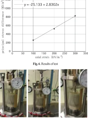
Triaxial compression means the loading in the three axis from all sides. For this purpose, the free space between the sample chamber and the device is liquid. Thus, we can get an extra uniform lateral pressure (Fig. 1).

Thanks to the uniform compression of the sample, geotechnical engineers can get the necessary

Back pressure Principal stress difference(max)

100 264.86

200 526.98

300 830.91

Slope of the straight linef0 25.135

Slope m0 2.8303

Angle of shear resistanceΦ 35.87

Cohesionc 12.84

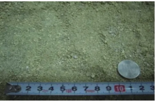
Fig.2.Pit sand Table 1.Physical properties of test sand

Fig. 3. Grain size distribution curve of test sand

Fig.4. Dependence of the relative vertical deformation of the vertical stress at constant lateral stress of 100, 200 and 300 kPa.

Fig. 5.Back pressure and principal stress difference Table 2. Physical properties of test sand

evidence, and the relationship between deformation and strength of the soil can be calculated as the final figures.

This test is greatly important in the construction of houses and buildings. Only on the basis of the obtained parameters the disigners can correctly calculate the foundation and the technical details of future construction.

Table 3. Physical of test sand Back pressure Principal stress difference(max)

100 369.46

200 684.02

300 999.85

Slope of the straight linef0 54.294

Slope m0 3.151

Angle of shear resistanceΦ 37.71

Cohesionc 26.65

3. EXPERIMENTAL PAET

In the experiment we used the Pit sand (Fig. 2).

Physical properties of the sand is shown in Table 1.

This test was conducted with sample of sand, a relative density of 75%, in different triaxial lateral pressures of 100, 200 and 300 kPa (Fig. 4).

Scheme test in consolidated-drained using trajectory compression was conducted. Test results are shown in Fig. 5, and the stress differences are shown in Table 4. We get the curve between principal stress difference and axial strain (Fig. 6).

The next test was conducted using samples of high density sand that density of 90%, and in different cell pressure of 100, 200 and 300 kPa (Fig. 7).

Scheme test consolidated-drained using trajectory compression was conducted. Test results are shown in Fig. 8, and the stress differences are shown in Table 5. We get the curve between principal stress difference and axial strain (Fig. 9).

Fig. 6. Results of test

Fig.7. Dependence of the relative vertical deformation of the vertical stress at constant lateral stress of 100, 200 and 300 kPa.

Fig. 8.Back pressure and principal stress difference

Fig. 9. Results of test

— 120 — 八戸工業大学紀要　第 34 巻 八戸工業大学紀要 第34巻

− 4−

4. CONCLUSIONS

The use of methods of triaxial compression to a large extent eliminates the shortcomings of current practice laboratory research when the same mechanical properties determined on several samples using various force loading conditions.

The tests in a triaxial compression will be possible more completely to understand behavior of the soil in the future based on the buildings or strucures in the laboratory. By comparing different sand density, it is shown that high

density sand has a lager principal stress difference.

5. ACKNOWLEDGEMENT

I’m grateful to Professors, Hachinohe Institute of Technology, A. Hasegawa and K. Kaneko, also for his geotechnical laboratory, where I was able to conduct experiments. And special thanks to researchers Geotechnical Institute, who helped me to carry out experiments. I have very fond memories about Japan, especially Hachinohe Institute of Technology in Hachinohe.

要 旨

筆頭著者バルジャン・カルダノバ氏（Balzhan Kaldanova）は、2014年10月26日から11 月28日まで、地盤工学、特に三軸圧縮試験に関する研究のために、八戸工業大学客員研究員と して来日した。 現職は、カザフスタンの首都アスタナ市にある国立ユーラシア大学の研究員で ある。大学院生小山直輝君と研究員橋詰豊氏の支援のもとで、砂の三軸圧縮試験を実施した。

この報告は、試験の概要と異なる相対密度の供試体について行った試験結果を示し、比較考察 したものである。

キーワード㻌㻦三軸圧縮試験、力学特性、最大主応力差、軸ひずみ、軸応力

5

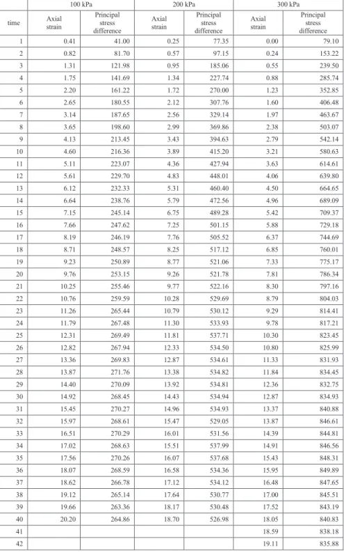
Table 4– Stress differences

100 kPa 200 kPa 300 kPa

time Axial

strain

Principal stress difference

Axial strain

Principal stress difference

Axial strain

Principal stress difference

1 0.41 41.00 0.25 77.35 0.00 79.10

2 0.82 81.70 0.57 97.15 0.24 153.22

3 1.31 121.98 0.95 185.06 0.55 239.50

4 1.75 141.69 1.34 227.74 0.88 285.74

5 2.20 161.22 1.72 270.00 1.23 352.85

6 2.65 180.55 2.12 307.76 1.60 406.48

7 3.14 187.65 2.56 329.14 1.97 463.67

8 3.65 198.60 2.99 369.86 2.38 503.07

9 4.13 213.45 3.43 394.63 2.79 542.14

10 4.60 216.36 3.89 415.20 3.21 580.63

11 5.11 223.07 4.36 427.94 3.63 614.61

12 5.61 229.70 4.83 448.01 4.06 639.80

13 6.12 232.33 5.31 460.40 4.50 664.65

14 6.64 238.76 5.79 472.56 4.96 689.09

15 7.15 245.14 6.75 489.28 5.42 709.37

16 7.66 247.62 7.25 501.15 5.88 729.18

17 8.19 246.19 7.76 505.52 6.37 744.69

18 8.71 248.57 8.25 517.12 6.85 760.01

19 9.23 250.89 8.77 521.06 7.33 775.17

20 9.76 253.15 9.26 521.78 7.81 786.34

21 10.25 255.46 9.77 522.16 8.30 797.16

22 10.76 259.59 10.28 529.69 8.79 804.03

23 11.26 265.44 10.79 530.12 9.29 814.41

24 11.79 267.48 11.30 533.93 9.78 817.21

25 12.31 269.49 11.81 537.71 10.30 823.45

26 12.82 267.94 12.33 534.50 10.80 825.99

27 13.36 269.83 12.87 534.61 11.33 831.93

28 13.87 271.76 13.38 534.82 11.84 834.45

29 14.40 270.09 13.92 534.81 12.36 832.75

30 14.92 268.45 14.43 534.94 12.87 834.93

31 15.45 270.27 14.96 534.93 13.37 840.88

32 15.97 268.61 15.47 529.05 13.87 846.61

33 16.51 270.29 16.01 531.56 14.39 844.81

34 17.02 268.63 15.51 537.99 14.91 846.56

35 17.56 270.26 16.07 537.68 15.43 848.31

36 18.07 268.59 16.58 534.36 15.95 849.89

37 18.62 266.78 17.12 534.12 16.48 847.65

38 19.12 265.14 17.64 530.77 17.00 845.51

39 19.66 263.36 18.17 530.48 17.52 843.19

40 20.20 264.86 18.70 526.98 18.05 840.83

41 18.59 838.18

42 19.11 835.88

— 122 — 八戸工業大学紀要　第 34 巻

八戸工業大学紀要 第34巻

− 6−

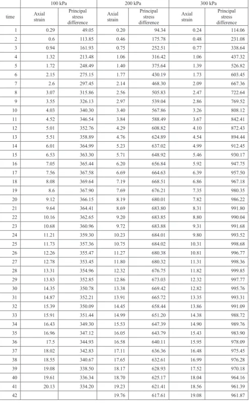
Table 5– Stress differences

100 kPa 200 kPa 300 kPa

time Axial

strain

Principal stress difference

Axial strain

Principal stress difference

Axial strain

Principal stress difference

1 0.29 49.05 0.20 94.34 0.24 114.06

2 0.6 113.85 0.46 175.78 0.48 231.08

3 0.94 161.93 0.75 252.51 0.77 338.64

4 1.32 213.48 1.06 316.42 1.06 437.32

5 1.72 248.49 1.40 375.64 1.39 526.82

6 2.15 275.15 1.77 430.19 1.73 603.45

7 2.6 297.45 2.14 468.30 2.09 667.36

8 3.07 315.86 2.56 505.83 2.47 722.64

9 3.55 326.13 2.97 539.04 2.86 769.52

10 4.03 340.30 3.40 567.86 3.26 808.12

11 4.52 346.54 3.84 588.49 3.67 842.41

12 5.01 352.76 4.29 608.82 4.10 872.43

13 5.51 358.89 4.76 624.89 4.54 894.44

14 6.01 364.99 5.23 637.02 4.99 912.45

15 6.53 363.30 5.71 648.92 5.46 930.17

16 7.05 365.44 6.20 656.84 5.92 947.75

17 7.56 367.58 6.69 664.63 6.39 957.50

18 8.08 369.64 7.19 668.51 6.86 967.18

19 8.6 367.90 7.69 676.21 7.35 980.35

20 9.12 366.15 8.19 680.01 7.82 986.22

21 9.64 364.41 8.69 683.80 8.31 991.80

22 10.16 362.65 9.20 683.85 8.80 990.04

23 10.68 360.96 9.72 683.88 9.31 991.68

24 11.21 359.30 10.23 684.01 9.80 993.52

25 11.73 357.36 10.75 684.02 10.31 998.68

26 12.26 355.47 11.27 680.38 10.81 996.77

27 12.78 353.45 11.80 680.32 11.31 998.36

28 13.31 354.96 12.32 676.75 11.82 999.85

29 13.83 352.85 12.86 673.03 12.32 997.77

30 14.35 350.78 13.38 669.42 12.82 995.76

31 14.87 352.21 13.91 665.72 13.35 993.31

32 15.39 350.09 14.45 658.44 13.86 991.09

33 15.91 351.44 14.99 651.20 14.38 988.72

34 16.43 349.30 15.53 647.39 14.90 989.76

35 16.96 347.12 16.05 643.79 15.43 983.90

36 17.5 344.93 16.58 640.11 15.95 978.09

37 18.02 342.83 17.11 636.36 16.48 975.45

38 18.55 340.67 17.65 632.61 16.99 976.28

39 19.08 338.50 18.17 628.93 17.52 970.18

40 19.61 336.34 18.70 625.17 18.04 964.16

41 20.13 334.20 19.23 621.41 18.56 961.39

42 19.76 617.61 19.08 961.87