- 83 - IEEE Workshop on Nonlinear Circuit NetworksDecember 7-8, 2018

(1)

Synchronization Phenomena in Coupled Nonlinear Oscillators Chains with Hourglass Structure

Takumi Nara, Daiki Nariai, Yoko Uwate and Yoshifumi Nishio Dept. Electrical and Electronic Engineering,

Tokushima University

2-1 Minami-Josanjima, Tokushima 7708506, Japan Email: { nara, nariai, uwate, nishio } @ee.tokushima-u.ac.jp

Abstract—In this study, we investigate synchronization phe-

nomena from circuit network, which is composed of several numbers of van der Pol oscillator chains. We use van der Pol oscillators which are coupled by resistors. We investigate how synchronization phenomena changes by changing the number of van der Pol oscillators. From the computer simulations, we observe relatively interesting synchronization phenomena.

I. I

NTRODUCTION

Synchronization phenomena are the most familiar phenomena that exist in nature and it has been studied in various fields, such as in electrical, in mechanics, in biological systems, ba- sically everywhere. Synchronization phenomena are observed everywhere in our life. For example, we can confirm flashing firefly lights, metronome, periodic swinging of candle flames, gate patterns of four-leg animals, beating rhythm of the heart and so on. Among them, van der Pol oscillators can observe phenomena similar to natural phenomena. Therefore we have been interested in coupled oscillators which synchronization phenomena from circuit network.

In this study, we investigate synchronization phenomena from a circuit network, which is composed of several numbers of van der Pol oscillator chains. The circuit model of van der Pol oscillator is shown in Fig. 1. This circuit consists of an inductor, a capacitor and a nonlinear resistance. From the computer simulations, we observe relatively interesting synchronization phenomena. We focus on synchronization phenomena in the coupled nonlinear circuits.

C L

Fig. 1. Circuit of van der Pol.

II. P

REVIOUS STUDY

Figure 2 shows the previous study circuit model. Bottom, middle and top are coupled with oscillators by resistors r.

Bottom several numbers of oscillator are coupled by resistors R

i

. Further, top several numbers of oscillator are coupled to ground via resistors R

a

through inductors. Middle oscillators

are not coupled with oscillators located in the horizontal di- rection but coupled vertically. In this network, we coupled the oscillators of bottom several numbers of oscillator in the chains to tend to produce in-phase synchronizations. Further, we coupled the oscillators of the top several numbers of oscillator in the chains to tend to produce anti-phase synchronizations.

Middle oscillators are coupled with bottom and top several numbers of oscillator. However, they are not coupled with the other chains.[1]

We define the bottom several numbers of oscillator as Osc

11

, Osc

12

, and Osc

1m

from the left. Further the middle several numbers of oscillator as Osc

21

, Osc

22

, and Osc

2m

from the left and the top several numbers of oscillator as Osc

31

, Osc

32

, and Osc

3m

from the left.

C L

ig12

vC12

iL12

C L

ig11

vC11

iL11

C L

ig13

vC13

iL13

C L C L C L

ig22

vC22

iL22

ig31

vC31 C

ig32

vC32 C

ig33

vC33 C

Ra Ra

Ri Ri

i³¹^b i³¹â i32b i³²â i³³^b i³³â r r

2L 2L 2L 2L 2L 2L

ig21

vC21

iL21 ig23

vC23

iL23

r r r

r

Fig. 2. Previous study system model.

First, we assume that the v − i characteristics of the nonlinear resistor in each oscillator are given by the follows:

i

_gn

= − g

₁

v

_n

+ g

₃

v

_n³

(1) where g

1

, g

3

> 0.

- 83 -

IEEE Workshop on Nonlinear Circuit Networks December 7-8, 2018

(2)

III. S

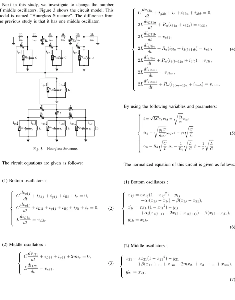
YSTEM MODEL

Next in this study, we investigate to change the number of middle oscillators. Figure 3 shows the circuit model. This model is named “Hourglass Structure”. The difference from the previous study is that it has one middle oscillator.

C L

ig12

vC12

i_L12

C L

ig11

vC11

i_L11

C L

ig13

vC13

iL13

C L

ig21

vC21

iL21

ig31

vC31 C

ig32

vC32 C

ig33

vC33 C

Ra Ra

Ri Ri

i³¹^b i31a i32b i³²^a i³³^b i³³^a r

r

2L 2L 2L 2L 2L 2L

r r

Fig. 3. Hourglass Structure.

The circuit equations are given as follows:

(1) Bottom oscillators :

 

 



 

 

C dv

c1j

dt + i

L1j

+ i

g1j

+ i

Ri

+ i

r

= 0, C dv

c1l

dt + i

L1l

+ i

g1j

+ i

Ri

+ i

Ri

+ i

r

= 0, L di

_L1k

dt = v

_c1k

.

(2)

(2) Middle oscillators :

 

 

 



C dv

c21

dt + i

L21

+ i

g21

+ 2mi

r

= 0, L di

L21

dt = v

c21

.

(3)

(3) Top oscillators :

 

 

 

 



C dv

c3k

dt + i

_g3k

+ i

_r

+ i

_3ka

+ i

_3kb

= 0, 2L di

L31a

dt + R

a

(i

31a

+ i

32b

) = v

c31

, 2L di

_L31b

dt = v

_c31

, 2L di

L3la

dt + R

a

(i

3la

+ i

_3(l+1)b

) = v

c3l

, 2L di

L3lb

dt + R

a

(i

_3(l₋_1)a

+ i

3lb

) = v

c3l

, 2L di

_L3ma

dt = v

_c3m

, 2L di

L3mb

dt + R

a

(i

_3(m₋_1)a

+ i

3mb

) = v

c3m

. (4)

By using the following variables and parameters:

 

 

 

 



t=√

LCτ, vkj=

√

g1

g3

xkj

ikj=

√

g1C

g3Lykj, ε=g1

√

C L αa=Ra

√

C L, αi= 1

Ri

√

L C, β= 1

r

√

L C.

(5)

The normalized equation of this circuit is given as follows:

(1) Bottom oscillators :

 

 

 

 



˙

x

1j

= εx

1j

(1 − x

1j2

) − y

1j

− α

i

(x

1j

− x

1l

) − β(x

1j

− x

21

),

˙

x

_1l

= εx

_1l

(1 − x

_1l²

) − y

_1l

+α

_i

(x

_1(l₋₁₎

− 2x

_1l

+ x

_1(l+1)

) − β(x

_1l

− x

₂₁

),

˙

y

1k

= x

1k

.

(6)

(2) Middle oscillators :

 

 

 



˙

x

₂₁

= εx

₂₁

(1 − x

₂₁²

) − y

₂₁

+β(x

₁₁

+ ... + x

_1m

− 2mx

₂₁

+ x

₃₁

+ ... + x

_3m

),

˙

y

21

= x

21

.

(7)

- 84 -

(3)

(3) Top oscillators :

 

 

 

 



˙

x

3k

= εx

3k

(1 − x

3k2

)

− (y

3ka

+ y

3kb

) − β(x

3k

− x

21

),

˙ y

_31a

= 1

2 { x

₃₁

− α

_a

(y

_31a

+ y

_32b

) } ,

˙ y

_31b

= 1

2 x

₃₁

,

˙ y

_3la

= 1

2 { x

_3l

− α

_a

(y

_3la

+ y

_3(l+1)b

) } ,

˙ y

3lb

= 1

2 { x

3l

− α

a

(y

3(l−1)a

+ y

3lb

) } ,

˙ y

3ma

= 1

2 x

3m

,

˙ y

3mb

= 1

2 { x

3m

− α

a

(y

_3(m₋_1)a

+ y

3mb

) } .

(8)

( j = 1, m ・ k = 1, 2, ..., m ・ l = 2, 3, ..., m − 1 ) . IV. S

IMULATION RESULTS

(A) Case of previous study

Figures 4 and 5 show the computer simulation results for the case of the previous study model. The circuit parameters are chosen as ε = 0.10, α

_a

= α

_i

= 0.50 and β = 0.02.

The bottom three oscillators are become in-phase synchronization and the top three oscillators are become anti-phase synchronization.

x₁₁ x₁₁ x₁₁ x₁₁

x₁₁ x₁₁

x₁₁ x₁₁ x₁₁

x₁₁ x₂₁

x₃₁

x₁₂ x₁₃ x₂₃ x₃₃

x₂₂ x₃₂

Fig. 4. Computer simulation results (phase shift) for previous study.

x₁₁ x12

x₃₃ x₁₃ x₂₁ x₂₂ x23

x₃₁ x₃₂

→τ

Fig. 5. Computer simulation results (time waveforms) for previous study.

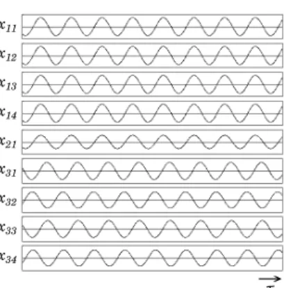
(B) Case of hourglass structure (m = 3)

Figures 6 and 7 show the computer simulation results for the case of hourglass structure. The circuit parameters are chosen at the same.

In comparison with (A), the phase shift with Osc

11

is approaching in-phase synchronization or anti-phase synchronization.

x

₁₁

x

₁₁

x

₁₁

x

₁₁

x

₁₁

x

₁₁

x

₁₁

x

₁₁

x

₁₂

x

₁₃

x

₂₁

x

₃₃

x

₃₂

x

₃₁

Fig. 6. Computer simulation results (phase shift) for hourglass structure (m= 3).

x₁₁

x₁₂

x₃₁ x₂₁ x₁₃

x₃₂

x₃₃

→τ

Fig. 7. Computer simulation results (time waveforms) for hourglass structure (m= 3).

(C) Case of hourglass structure (m = 4)

Figures 8 and 9 show the computer simulation results for the case of hourglass structure. The circuit parameters are chosen at the same.

In comparison with (B), we increase one oscillator to the top and bottom. As (A) and (B), the bottom oscillators are in-phase synchronization and the top oscillators are anti-phase synchronization. However, in comparison with (B), the top oscillators are not in-phase synchronization and anti-phase synchronization with Osc

11

.

x₁₁ x₁₁ x₁₁ x₁₁ x₁₁

x₁₁ x₁₁ x₁₁ x₁₁

x₁₁ x₁₂ x₁₃ x₁₄ x₂₁

x₃₁ x₃₂ x₃₃ x₃₄

Fig. 8. Computer simulation results (phase shift) for hourglass structure (m= 4).

- 85 -

(4)

x₁₁

x₁₂

x₁₃

x₁₄

x₂₁

x₃₁

x₃₂

x₃₃

x₃₄

→τ

Fig. 9. Computer simulation results (time waveforms) for hourglass structure (m= 4).

From Figs. 6 and 8 there is the difference in the synchronization phenomena of the top oscillators. The top oscillators of all results are anti-phase synchronization. However, looking at the result of phase shift with Osc

₁₁

, when the value of m is an odd number, the phase shift with Osc

11

is approaching the in-phase synchronization or anti-phase synchronization, and when the value of m is an even number, the different synchronization was observed in Osc

11

and top oscillators.

V. C

ONCLUSIONS

In this study, we have investigated synchronization phenomena observed by circuit networks, which are composed of several numbers of van der Pol oscillator chains. By the computer simulations, we could obtain of results that the bottom oscillators observe in-phase synchronization and the top oscillators observe anti-phase synchronization. Further, we could observe synchronization phenomena by changing with the value of m .

In the future works, we will investigate synchronization phenomena using other parameters. Further, when the value of m is an odd number or an even number, the synchronization phenomena occur in the Osc

₂₁

of the middle oscillator and guess some cause. Therefore, we investigate this case in detail. Further, in this study, we have investigated oscillators connected symmetrically to left and right, but we would like to investigate circuit models that are connected asymmetrically to left and right by increasing the number of oscillators in the middle.

R

EFERENCES

[1] K. Matsumura, T. Nagai, Y. wate and Y. Nishio, “Analysis of Synchro- nization Phenomenon in Coupled Oscillator Chains,” Proceedings of IEEE International Symposium on Circuits and Systems (ISCAS’12), pp.620- 623, May 2012.

[2] D. Nariai,M. Tran, Y. Uwate and Y. Nishio, “Synchronization in Two Rings of Coupled Three van der Pol Oscillators,” Proceedings of RISP International Workshop on Nonlinear Circuits, Communications and Signal Processing (NCSP’17), pp.289-292, FEb.2017.

[3] V. Hien,M. Tran, Y. Uwate, Y. Nishio, “Effect of Changing Coupling Strength to Synchronization Phenomena in Coupled van der Pol Oscilla- tors,” Proceedings of RISP International Workshop on Nonlinear Circuits, Communications and Signal Processing (NCSP’18), pp. 148-151, Mar.

2018.

[4] T. Matsunashi, D. Nariai, Y. Uwate and Y. Nishio, “Synchronization Phenomena in a Ring of van der Pol Oscillators Coupled by Time-Varying Resistor,” Proceedings of RISP International Workshop on Nonlinear Circuits, Communications and Signal Processing (NCSP’18), pp. 168- 171, Mar. 2018.

- 86 -