RIMS-1713
On the equivalence of parabolic Harnack inequalities and heat kernel estimates
By
Martin T. BARLOW, Alexander GRIGOR’YAN and Takashi KUMAGAI
March 2011
R ESEARCH I NSTITUTE FOR M ATHEMATICAL S CIENCES
On the equivalence of parabolic Harnack inequalities and heat kernel estimates
Martin T. Barlow
⇤Department of Math.
University of British Columbia Vancouver V6T 1Z2, Canada
Alexander Grigor’yan
†Department of Math.
University of Bielefeld 33501 Bielefeld, Germany Takashi Kumagai
‡RIMS
Kyoto University Kyoto 606-8502, Japan
3 March 2011
Abstract
We prove the equivalence of parabolic Harnack inequalities and sub-Gaussian heat kernel estimates in a general metric measure space with a local regular Dirichlet form.
Key Words and Phrases. Harnack inequality, heat kernel estimate, caloric function, metric measure space, volume doubling, Dirichlet space
Short title. Parabolic Harnack inequalities and heat kernel estimates
2010 Mathematics Subject Classification. Primary 58J35; Secondary 60J35, 31C25.
Contents
1 Introduction 2
2 Framework and background material 5
2.1 General setup . . . 5 2.2 Caloric functions . . . 6
⇤Research partially supported by NSERC (Canada)
†Research partially supported by SFB 701 of the German Research Council (DFG)
‡Research partially supported by the Grant-in-Aid for Scientific Research (B) 22340017 (Japan)
3 Main result 9
3.1 The Harnack inequality . . . 9
3.2 The statement of the main result . . . 11
4 Proof of Theorem 3.1 12 4.1 Proof of (a))(b) (w-HKE implies w-LLE) . . . 12
4.2 Proof of (b))(c) (w-LLE implies w-PHI) . . . 15
4.2.1 Oscillation inequality and the H¨older continuity . . . 15
4.2.2 Obtaining the Harnack inequality . . . 19
4.3 Proof of (c))(a) (w-PHI implies w-HKE) . . . 24
4.3.1 A technical lemma . . . 24
4.3.2 Oscillation inequality and the H¨older continuity . . . 25
4.3.3 Existence of the heat kernel and on-diagonal upper bound . . 27
4.3.4 Near diagonal lower bound . . . 31
4.3.5 Integrated upper bound . . . 35
4.3.6 Pointwise o↵-diagonal upper bound . . . 38
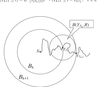
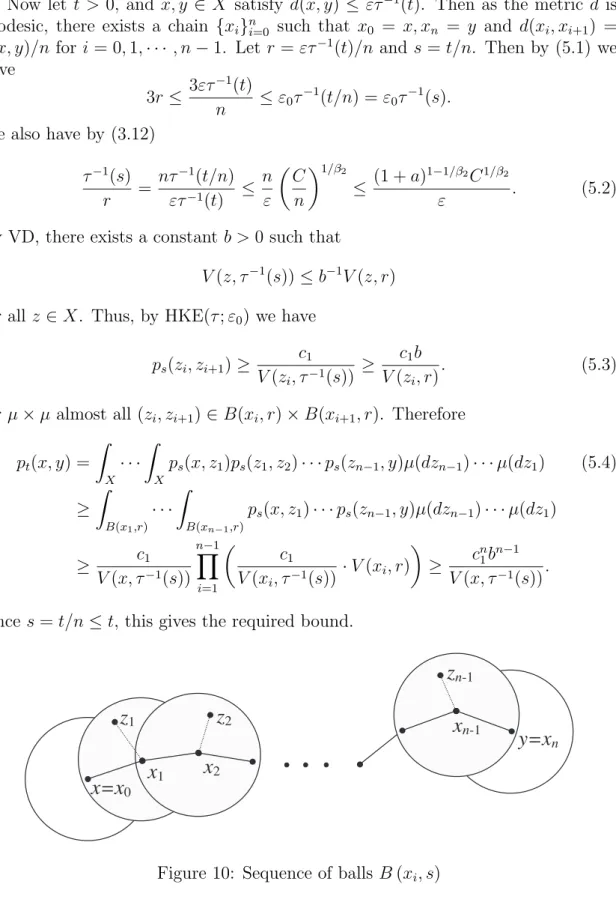
5 Proof of Theorem 3.2 40
6 Example 44
1 Introduction
The classical Harnack inequality says that if u is a non-negative harmonic function in a ball B(x, R) in Rn then
sup
B(x,12R)
uC inf
B(x,12R)u
where the constant C depends only on n. The same inequality holds for solutions of a uniformly elliptic equation
Lu:=
Xn
i,j=1
@
@xi
✓
aij(x) @u
@xj
◆
= 0
where now the constantC depends only on n and on the ellipticity constant of the operator L. The Harnack inequality has proven to be a powerful tool in analysis of elliptic PDEs. For example, it can be used to obtain the H¨older continuity of solutions, convergence properties of sequences of solutions, estimates of fundamental solutions, boundary regularity, etc.
Aparabolicversion of the Harnack inequality, which was discovered by Hadamard, says that if u= u(t, x) is a non-negative solution of the heat equation @u@t = u in a cylinder (0, T)⇥B(x, R) where T =R2, then
sup (14T,12T)⇥B(x,12R)
u(t, x)C inf
(34T,T)⇥B(x,12R)u(t, x), (1.1)
where again C depends only on n. By a theorem of Moser [29], the same inequality holds also for solutions of the parabolic equation @u@t = Lu where the constant C depends in addition on the ellipticity constant of L (here the coefficients of L are allowed to depend on t as well). A spectacular application of Moser’s Harnack inequality was the proof by Aronson [1] of the Gaussian estimates of the heat kernel pt(x, y) of the equation @u@t =Lu:
C2
tn/2 exp c2|x y|2 t
!
pt(x, y) C1
tn/2 exp c1|x y|2 t
!
. (1.2) To be more precise, the Harnack inequality was used in [1] to prove the lower bound in (1.2), while the upper bound was obtained using an additional argument. Even earlier Littman, Stampaccia and Weinberger [27] used the elliptic Harnack inequality of Moser to obtain estimates of fundamental solution of the operator L. It was first observed by Landis that conversely, if one had proper two sided estimates of the fundamental solution of L then one could deduce the Harnack inequality, although in a highly elaborate manner. The argument of Landis was further developed by Krylov and Safonov [24] in the context of parabolic equations, and then was brought by Fabes and Stroock [11] to a final, transparent form.
In the meantime, the development of analysis on Riemannian manifold raised similar questions in the geometric context. Let now be the Laplace-Beltrami op- erator on a complete non-compact Riemannian manifoldX. Then one can consider the associated Laplace equation u = 0 and heat equation @u@t = u and ask the same questions as above. It was quickly realized that the Harnack inequalities and heat kernel bounds require quite strong restrictions on the geometry of the mani- fold. The questions above are transformed in the context of the heat equation as follows: under what geometric hypotheses can one obtain analogues of the parabolic Harnack inequality (1.1) and the heat kernel bounds (1.2) on Riemannian manifold and whether these two properties are equivalent? The first breakthrough result in this direction is the following estimate of Li and Yau [26]: if the Ricci curvature of X is non-negative then the heat kernel pt(x, y) admits the bounds
pt(x, y)⇣ C V x,p
t exp
✓
cd2(x, y) t
◆
(1.3) where d(x, y) is the geodesic distance, V (x, r) is the Riemannian volume of the geodesic ballB(x, r), and⇣means that both inequalities with and take place but possibly with di↵erent values of positive constants C, c. In fact, Li and Yau proved the uniform Harnack inequality (1.1) for solutions of the heat equations onX, and then used it to obtain (1.3) as in Aronson’s proof. Similar estimates for certain unbounded domains inRnwith Neumann boundary conditions were obtained by a di↵erent method by Gushchin [20].
An analysis of the arguments of Fabes and Stroock [11] and Aronson [1] shows the following:
1. If the killed heat kernel on X satisfies the lower bound pB(xt 0,R)(x, y) c
V x0,p
t for all x, y 2B⇣ x0, "p
t⌘
(1.4)
for all x0 2 X and 0 < t "R2, for some positive constants ", c, then the Harnack inequality (1.1) holds.
2. If the Harnack inequality (1.1) holds then also the estimates (1.3) are satisfied.
It is not difficult to show that (1.3) implies (1.4). Hence, we obtain the equiva- lence
(1.1),(1.3),(1.4). (1.5)
Note that the proof of the equivalence (1.5) requires also the following general prop- erties of Riemannian manifolds:
(a) For any y 2 X, the function f(x) = d(x, y) has its gradient bounded by 1, that is,|rf| 1. (This is used to obtain the upper bound in (1.3))
(b) For any couple x, y 2X, there is a geodesic connectingxand y. (This is used to obtain the lower bound in (1.3)).
During the past two decades the study of heat kernels and Harnack inequalities has gained a new momentum from analysis on fractals and more general metric measure spaces. Let (X, d) be a locally compact metric space and µ be a Radon measure onX with full support. We refer to the triple (X, d, µ) as a metric measure space. As it was shown in [7], [4], [12] various classes of fractals (X, d, µ) admit a natural Laplace operator, whose heat kernel satisfies the following estimates
pt(x, y)⇣ C
t↵/ exp c
✓d (x, y) t
◆ 11!
, (1.6)
where↵ >0 and >1 are positive parameters. In fact,↵is the Hausdor↵ dimension of (X, d), and is also the exponent of the volume growth function, that is,
µ(B(x, r))⇣Cr↵ (1.7)
whereB(x, r) is the metric ball of d. The parameter is called the walk dimension of the associated di↵usion process; one has always 2. The Harnack inequality (1.1) is also satisfied on such spaces, although the relation between the time and space dimensions T and R has to be changed to T =R .
Under the assumptions that (X, d) is a length space and the heat kernel on X is a continuous function, it was shown by Hebisch and Salo↵-Coste [22], that the Harnack inequality withT =R is equivalent to the following heat kernel estimates:
pt(x, y)⇣ C
V (x, t1/ ) c
✓d (x, y) t
◆ 11!
, (1.8)
whereV (x, r) =µ(B(x, r)). It is clear that under the condition (1.7), the estimate (1.8) is the same as (1.6).
The purpose of this paper is to study the equivalence of the heat kernel estimates and Harnack inequalities in a general setting without additional assumption on the
metric d, and without the continuity of the heat kernel. In particular we do not assume thatdis a geodesic metric. Our main result is an analogue of the equivalence (1.5) in a general setup. Our weaker hypotheses makes our arguments much more technical but in return allows much more flexibility in applications. We remark that typically the continuity of the heat kernel cannot be established a priori. To deduce the Harnack inequality from the heat kernel estimates, we use a modification of the argument of Fabes and Stroock [11]. To obtain heat kernel estimates from the Harnack inequality, we use the following.
• For the on-diagonal upper bound – an adaptation of the argument of Aronson [1], although the singularity of the setting requires much more work.
• For the lower bounds – a new argument, based on [9], which allows one to avoid gluing solutions in time as in [1].
• For the o↵-diagonal upper bounds – a modification of the argument of Hebisch and Salo↵-Coste [22]. Note that the classical argument of Aronson does not work because the estimate|rd| 1 is no longer true.
We do not touch here on the interesting question of deducing either the Harnack inequality or the heat kernel bounds from some simpler properties, and refer the reader to [6], [14], [31], [32] and references therein.
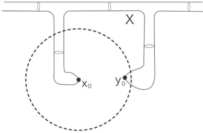
Finally, note that there are various examples of distances that are not geodesic.
For example, the resistance metric that gives an e↵ective resistance between two points is an important metric for the heat kernel estimates for di↵usions on fractals (see for example [21]), and the external metric is often useful for global analysis on metric spaces (see Fig. 11 in Section 6 where 2-dimensional Riemannian manifold X is embedded in R3; the external metric is then the Euclidean metric onR3).
2 Framework and background material
2.1 General setup
Let (X, d) be a locally compact complete separable metric space. Let µ be a Borel measure onX with full support, that is, 0 < µ(⌦)<1for every non-void open set
⌦⇢X. We will refer to such a triple (X, d, µ) as ametric measure space.
Let (E,F) be a regular strongly local Dirichlet form onL2(X, µ). The regularity means that the intersection F \C0(X) is dense both in F and C0(X), where the latter is the space of all compactly supported continuous functions on X with sup- norm, and the norm ofF is given by the inner product (f, g) +E(f, g). The strong locality means that E (u, v) = 0 whenever u, v are functions from F with compact supports such that u = const in an open neighborhood of suppv. We refer to the quadruple (X, d, µ,E) as a metric measure Dirichlet space. For any open set ⌦⇢X, F⌦is defined as the closure inF of the set of all functions fromF that are compactly supported in ⌦. It is known that (E,F⌦) is a regular strongly local Dirichlet form onL2(⌦, µ) (see [13, Section 4.4]).
Denote byLthe (negative definite) generator ofE, which is a self-adjoint operator inL2 such that
E(f, g) = (Lf, g)L2
for all f 2 dom (L) and g 2 F. Let {Pt}t 0 be the heat semigroup of the form (E,F), that is, Pt =etL where etL is defined by the spectral theory as an operator inL2.
For any open set ⌦ ⇢ X, denote by L⌦ the generator (E,F⌦) and by Pt⌦ t 0 the associated heat semigroup. Let Y = {Yt}t 0,{Px}x2X be the Hunt process associated with the Dirichlet form (E,F) (see [13, Theorem 7.2.1]). Since E is strongly local, by [13, Theorem 7.2.2]Y is a di↵usion.
For example, for Brownian motion in Rd, we have E(f, g) = 1
2 Z
Rd
(rf,rg)dx,
F =W1 Rd , and L= /2 with domain dom (L) = {f 2 F : f 2L2}.
2.2 Caloric functions
We need to define what it means that a function u(t, x) is a caloric function in a cylinder I ⇥⌦, where I is an interval in R and ⌦ is an open subset of X. In the classical case of analysis in Rn, a caloric function u(t, x) is a solution of the heat equation @u@t = u. In the abstract setting there are various definitions; for our purposes, any definition will do as long as it satisfies the following properties:
1. The set of all caloric functions in I⇥⌦ is a linear space over R.
2. IfI0 ⇢I and ⌦0 ⇢⌦ then any caloric function inI⇥⌦ is also a caloric function inI0⇥⌦0.
3. For any g 2 L2(⌦, µ), the function (t, x) 7! Pt⌦g(x) is a caloric function in R+⇥⌦.
4. If ⌦ is relatively compact then a constant function in ⌦ is the restriction to ⌦ of a time independent caloric function in R+⇥⌦.
5. (Super-mean value inequality) For any non-negative caloric function u(t, x) in R+⇥⌦, the following inequality holds: u(t,·) Pt s⌦ u(s,·) for all 0 < s < t.
(We remark that when we write inequalities of this kind, we intend them to be for functions inL2(X, µ) rather than pointwise.)
We now give one definition of caloric functions that satisfies all these require- ments. Write for simplicity L2 =L2(X, µ), and let I be an interval in R. We say that a function u : I ! L2 is weakly di↵erentiable at t0 2 I if for any f 2 L2, the function (u(t), f) is di↵erentiable at t0 (where the brackets stand for the inner product in L2), that is, the limit
t!tlim0
✓u(t) u(t0) t t0
, f
◆
exists. By the principle of uniform boundedness, in this case there is a function w2L2 such that
tlim!t0
✓u(t) u(t0) t t0 , f
◆
= (w, f)
for all f 2L2. We refer to the function w as the weak derivative of the function u att0 and write w=u0(t0). Of course, we have the weak convergence
u(t) u(t0) t t0
* u0(t0).
Similarly, one can introduce the strong derivative ofuif u(t)t tu(t0 0) converges tou0(t0) in the norm topology ofL2.
Definition. Consider a function u:I ! F, and let ⌦ be an open subset ofX. We say that uis a subcaloric function in I⇥⌦ ifuis weakly di↵erentiable in the space L2(⌦) at any t2I and, for any non-negativef 2 F⌦ and for any t 2I,
(u0, f) +E(u, f)0. (2.1)
Equivalently, u is subcaloric if (u, f) is di↵erentiable in t 2 I for any f 2 L2(⌦), and
(u, f)0+E(u, f)0 for anyf 2 F⌦. (2.2) Similarly one defines the notions of supercaloric functions and caloric functions; for the latter the inequalities (2.1) and (2.2) become equalities.
Clearly, the properties 1 and 2 above are satisfied. In what follows, we check 3 5.
Example 2.1 (i) Let us verify that, for any g 2 L2(⌦, µ), the function u(t,·) = Pt⌦g is a caloric function in R+⇥⌦. Note first that u(t,·) 2 F⌦ ⇢ F. Next, let {E } be the spectral resolution of L⌦. Then we have, for any f 2L2(⌦),
(u(t,·), f) = Pt⌦g, f = Z 1
0
e td(E g, f) whence, for any t >0,
(u(t,·), f)0 =
Z 1
0
e td(E g, f)
(the integral in the right hand side converges locally uniformly int >0 because the function 7! e t is bounded). On the other hand, for any f 2 F⌦, we have
E(u(t,·), f) = L⌦Pt⌦g, f = ⇣
(L⌦etL⌦)g, f⌘
= Z 1
0
e td(E g, f), whence
(u, f)0+E(u, f) = 0, (2.3)
that is,u is a caloric function.
(ii) Let ⌦ be relatively compact. Then there is a cuto↵ function of ⌦, that is, a function u 2 C0(X)\ F such that u ⌘ 1 in a neighborhood of ⌦. We claim that the function (t, x)7!u(x) is caloric in R⇥⌦. Indeed, anyf 2C0(⌦)\ F we have E(u, f) = 0 by the strong locality, and this identity extends by continuity to all f 2 F⌦. Sinceu0 = 0, the equation (2.3) is trivially satisfied, so that u(x) is a time independent caloric function inR⇥⌦.
The following maximum principle was proved in [18] (see also [15] for the case of the strong time derivative). For any real a, set a+ = max (a,0).
Lemma 2.2 Fix T 2 (0,1], an open set ⌦ ⇢ X, and let u : (0, T) ! F be a subcaloric function in (0, T)⇥⌦. Assume in addition that u satisfies the boundary condition
u+(t,·)2 F⌦ for all t 2(0, T) (2.4) and the initial condition
u+(t,·)L2!(⌦)0as t!0.
Then u+ = 0 in (0, T)⇥⌦, so that u0 in (0, T)⇥⌦.
Remark. The condition (2.4) can be verified in applications using the following result from [15]: ifu2 F and uv for somev 2 F⌦ then u+ 2 F⌦.
Finally, we can establish the super-mean value inequality.
Corollary 2.3 Let f 2 L2+(⌦) and u be a non-negative supercaloric function in (0, T)⇥⌦ such that u(t,·)L2!(⌦)f as t!0. Then, for any t 2(0, T),
u(t,·) Pt⌦f in ⌦. (2.5)
In particular, for all 0< s < t < T,
u(t,·) Pt s⌦ u(s,·) in ⌦. (2.6) Proof. Consider the functionv =Pt⌦f u, which by property 2 above is a weak subsolution in (0, T)⇥⌦. Since f 2L2,
v(t,·)L2!(⌦)0 as t!0 and, for any t >0,
v(t,·)Pt⌦f.
Since Pt⌦f 2 F⌦, we conclude by the Remark above that v+ 2 F⌦. By Lemma 2.2, we obtain v 0, which proves (2.5). Inequality (2.6) follows from (2.5) with f =u(s,·).
We note that an alternative approach to define caloric functions and develop a parabolic potential theory is via time dependent Dirichlet forms. Such forms can be defined by integrating time derivatives of space-time functions and the original
Dirichlet forms over the time variable. Roughly speaking, for a parabolic cylinder Q:=I⇥B(x0, R),u(t, x) :Q!R is a caloric function in Qif
Z
J
h Z f(t, x)u0(t, x)µ(dx) +E(f(t,·), u(t,·))i
dt= 0,
for all compact subinterval J ⇢ I and f : I ⇥X ! R so that f(t,·) has compact support in B(x0, R) for a.e. t 2 I. Time dependent Dirichlet forms are no longer symmetric and time derivatives should be considered in the distribution sense. We do not pursue this approach here, but remark that there is are unpublished lecture notes [30] that discuss the theory of time dependent Dirichlet forms.
3 Main result
Consider metric balls
B(x, R) ={y:d(x, y)< R}, and set
V(x, R) = µ(B(x, R)).
We assume in the sequel that all ballsB(x, R) are relatively compact for all x2X andR >0. In particular, the functionV (x, R) is finite and positive. For anyx2X and T, R >0, we define the cylinder
Q(x, T, R) = (0, T)⇥B(x, R) as a subset of R⇥X.
3.1 The Harnack inequality
We introduce here the Harnack inequality and other necessary properties for caloric functions on metric measure Dirichlet spaces. Let ⌧ : (0,1) ! (0,1) be a con- tinuous strictly increasing bijection that satisfies the following property: there exist 1< 1 2 <1and C >0 such that, for all 0< rR <1,
C 1
✓R r
◆ 1
⌧(R)
⌧(r) C
✓R r
◆ 2
. (3.1)
It follows that the inverse function ⌧ 1 satisfies the following condition: for all 0< tT < 1,
✓T Ct
◆1/ 2
⌧ 1(T)
⌧ 1(t)
✓CT t
◆1/ 1
. (3.2)
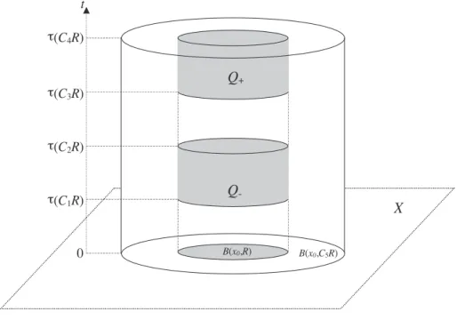
Definitions. We say that a metric measure Dirichlet space X satisfies the weak parabolic Harnack inequality with the rate function⌧ (for short w-PHI(⌧)) if there exist constants 0 < C1 < C2 < C3 < C4, C5 > 1 and C6 > 0 such that, for any
non-negative bounded caloric function u(t, x) in any cylinder Q(x0, ⌧(C4R), C5R), the following inequality is satisfied
ess sup
Q
uC6 ess inf
Q+
u, (3.3)
where
Q+ : = (⌧(C3R), ⌧(C4R))⇥B(x0, R) (3.4) Q : = (⌧(C1R), ⌧(C2R))⇥B(x0, R). (3.5) (See Fig. 1).
We say that X satisfies the strong parabolic Harnack inequality with the rate function⌧ (shortly, s-PHI(⌧)) if, for any choice of constants 0< C1 < C2 < C3 < C4 and C5 > 1, there exists C6 = C6(C1, ..., C5) > 0 such that w-PHI(⌧) holds with this set of constants.
It is immediate that s-PHI(⌧) implies w-PHI(⌧). The di↵erence between these strong and weak PHI is one of the main topics of this paper. We remark that this di↵erence has not been remarked on before since in the classical situation when
⌧(t) =t2 (ort with >2) and the metric is geodesic, a standard chaining argument shows that w-PHI(⌧) implies s-PHI(⌧). See Theorem 3.2 below for a generalization of this to ⌧ satisfying (3.1).
τ(C4R)
Q- Q+
B(x0,R)
0 t
B(x0,C5R)
τ(C3R)
τ(C2R)
τ(C1R) X
Figure 1: Cylinders Q+ and Q
In the following definitions we use the parameters 1 and 2 from (3.1). Also,
⌧ 1 denotes the inverse function of the ⌧.
Definitions. (i) We say thatXsatisfies HKE(⌧;"), where" 2(0,1) is a parameter, if{Pt}possesses a transition densitypt(x, y) that satisfies the following inequalities:
pt(x, y) c1
V(x, ⌧ 1(t))exp c2
✓⌧(d(x, y)) t
◆1/( 2 1)!
(3.6) for all t >0 and µ⇥µ-almost all (x, y)2X⇥X, and
pt(x, y) c3
V(x, ⌧ 1(t)), (3.7)
for all t >0 and µ⇥µ-almost all (x, y)2X⇥X with
d(x, y)"⌧ 1(t), (3.8)
wherec1, c2, c3 =c3(") are positive constants.
(ii) We say that X satisfies w-HKE(⌧) if HKE(⌧;") is satisfied for some " >0.
(iii) We say thatX satisfies s-HKE(⌧) if HKE(⌧;") is satisfied for all "2(0,1).
(iv) We say thatX satisfies f-HKE(⌧) if{Pt}possesses the transition densitypt(x, y) that satisfies (3.6) and the lower bound
pt(x, y) c3
V(x, ⌧ 1(t))exp c4
✓⌧(d(x, y)) t
◆1/( 2 1)!
, (3.9)
for all t >0 and µ⇥µ-almost all x, y 2X.
(v) We say that X satisfies LLE(⌧;"), where " 2 (0,1) is a parameter, if for all x0 2X and R >0, there exists a transition density ptB(x0,R)(x, y) of {PtB(x0,R)}that satisfies the estimate
pB(xt 0,R)(x, y) c5
V(x0, ⌧ 1(t)), (3.10) for all 0 < t ⌧("R) and µ-almost all x, y 2 B(x0, "⌧ 1(t)), with some positive constantc5.
(vi) We say that X satisfies w-LLE(⌧) if LLE(⌧;") is satisfied for some" 2(0,1).
(vii) We say that X satisfies s-LLE(⌧) if LLE(⌧;") is satisfies for all "2(0,1).
Here the abbreviation ‘HK’ stands for ‘heat kernel’ estimates, ‘w-’ stands for
‘weak’, ‘s-’ stands for ‘strong’, ‘f-’ stands for ‘full’, and LLE stands for ‘local lower estimate’.
3.2 The statement of the main result
We say that a metric measure space (X, d, µ) satisfies the volume doubling property VD, if there exists a constant C such that
V(x,2R)CV(x, R) for all x2X, R >0. (VD) It is easy to see that VD implies the following; there exist CVD, >0 such that
V(x, R)CVDV(y, r)
✓d(x, y) +R r
◆
, for all x, y 2X,0< rR. (3.11)
Our main result is as follows.
Theorem 3.1 Let(X, d, µ,E)be a metric measure Dirichlet space and assume that all metric balls are relatively compact and VD is satisfied. Then the following con- ditions are equivalent:
(a) X satisfiesw-HKE(⌧).
(b) X satisfies w-LLE(⌧).
(c) X satisfies w-PHI(⌧).
Let us emphasize that in this paper we never assume that (E,F) is conservative.
We say that a metric space (X, d) is geodesic if, for any couple x, y 2 X, there exists a (not necessarily unique) geodesic path, that is, a continuous path connecting the pointsx, y and such that, for any pointz on this path, d(x, z)+d(z, y) = d(x, y).
The following statement refines Theorem 3.1 in the case of a geodesic space.
Theorem 3.2 Let(X, d, µ,E)be a metric measure Dirichlet space and assume that all metric balls are relatively compact and the metric is geodesic. Assume also that the function ⌧ satisfies the condition1
✓R r
◆ 1
⌧(R)
⌧(r) C
✓R r
◆ 2
, 0< rR. (3.12)
The following are equivalent:
(a) X satisfies s-HKE(⌧).
(a0) X satisfies VD and w-HKE(⌧).
(a00) X satisfies f-HKE(⌧).
(b) X satisfies VD and s-LLE(⌧).
(b0) X satisfiesVD and w-LLE(⌧).
(c) X satisfies s-PHI(⌧).
(c0) X satisfies w-PHI(⌧).
Remark. Theorem 3.2 shows that s-LLE, s-HKE and s-PHI are equivalent provided the metric d is geodesic. Without the latter assumption the statement of Theorem 3.2 is not true in general. See Section 6 for an example of a space that satisfies s-HKE but neither s-PHI nor s-LLE.
4 Proof of Theorem 3.1
4.1 Proof of (a) ) (b) (w-HKE implies w-LLE)
We prove here that VD + w-HKE(⌧;") implies w-LLE(⌧). Let us first show that the heat semigroupPtB possesses the heat kernel for any ballB =B(x0, R). Indeed, by
1Note that (3.12) is stronger than (3.1) since the coefficient in the left hand side inequality is 1 rather thanC 1.
the upper bound (3.6) and (3.11) we have ess sup
x,y2B
pt(x, y)sup
x2B
c1
V(x, ⌧ 1(t)) c01 V(x0, r)
✓ 2R
⌧ 1(t)
◆
=:F (t). (4.1) Therefore, for any non-negative functionf 2L1(B) and µ-almost all x2B,
PtBf(x)Ptf(x) = Z
B
pt(x, y)f(y)dµ(y)F(t)kfkL1.
Hence, the semigroup PtB is L1 !L1 ultracontractive, which implies the existence of the heat kernel pBt (see [5], [8], [10], [16]).
By [15, Lemma 4.18], for any open set U ⇢X and any compact set K ⇢U, for any non-negative function f 2L2(X, µ) and any t >0, the following holds.
Ptf(x)PtUf(x) + sup
s2[0,t]
ess sup
Kc
Psf, (4.2)
for µ-almost all x 2 X. Let us apply this inequality with U = B :=B(x0, R) and K =B(x0, R/2). Fix some 0 < r < R/4 to be specified later on, set A =B(x0, r) and letf be a non-negative function from L1(A). We have
sup
s2[0,t]
ess sup
z2Kc Psf(z) = sup
s2(0,t]
ess sup
z2Kc
Z
A
ps(z, y)f(y)dµ(y)MkfkL1, where
M := sup
s2(0,t]
ess sup
z2Kc, y2Aps(z, y) (4.3)
(note that the value s = 0 can be dropped from sups2[0,t] because P0f = f and ess sup
z2Kc
f(z) = 0).
Multiplying (4.2) by a non-negative function g 2 L1(A) and integrating, we
obtain Z
A
(Ptf)g dµ Z
A
PtBf g dµ+MkfkL1kgkL1, which is equivalent to
Z
A
Z
A
pt(x, y)f(y)g(x)dµ(x)dµ(y) Z
A
Z
A
pBt (x, y)f(y)g(x)dµ(x)dµ(y) +MkfkL1kgkL1.
Dividing by kfkL1kgkL1 and taking inf in all test functions f, g, we obtain ess inf
x,y2A pt(x, y) ess inf
x,y2A pBt (x, y) +M. (4.4)
By the definition of w-LLE(⌧), we need to estimate ess inf
x,y2A pBt (x, y) from below assuming
t⌧("R) and r "⌧ 1(t), (4.5)
for some" 2(0,1).For that, we estimate the left hand side of (4.4) from below and M from above. The value of "will be chosen small enough to satisfy a number of re- quirements. From the beginning we can assume that" <1/4 and that w-HKE(⌧;") is satisfied. Then we have by (3.7)
ess inf
x,y2A pt(x, y) c3
V(x, ⌧ 1(t)). (4.6)
To estimate M from above, observe that, for allz 2Kc and y2A, d(z, y) R
2 r R
4. Also, for anyst, using" <1/4, we obtain by (3.1)
⌧(d(z, y)) s
⌧(R/4)
s C 1
✓ R 4⌧ 1(s)
◆ 1
.
Hence, for all 0< st and µ-almost all z 2Kc and y2A, we have by (3.6) ps(z, y) c1
V(y, ⌧ 1(s))exp c2
✓⌧(d(z, y)) s
◆1/( 2 1)!
c1
V(x0, ⌧ 1(t))
V(x0, ⌧ 1(t))
V(y, ⌧ 1(s)) exp c02
✓ R
⌧ 1(s)
◆ 1/( 2 1)!
C
V(x0, ⌧ 1(t))
✓ R
⌧ 1(s))
◆
exp c02
✓ R
⌧ 1(s)
◆ 1/( 2 1)! , where we have used (3.11) and ⌧ 1(t)R. Note that by (4.5)
R
⌧ 1(s) " 1. Using the fact that, for positive a, b,
⇠aexp c2⇠b !0 as ⇠! 1, we conclude that if " is small enough then
ps(z, y) c3/2 V (x0, ⌧ 1(t)), wherec3 is the constant from (4.6). It follows that also
M c3/2 V (x0, ⌧ 1(t)), which together with (4.4) and (4.6) implies
ess inf
x,y2A pBt (x, y) c3/2 V(x0, ⌧ 1(t)), which was to be proved.
4.2 Proof of (b) ) (c) (w-LLE implies w-PHI)
Here we prove that VD + LLE(⌧;") implies w-PHI(⌧). The argument mostly fol- lows [11, Section 5], with modifications that are appropriate to the present setting.
Observe first that LLE(⌧;") implies
pB(xt 0,R)(x, y) c6
V(x0, R), (4.7)
forµ⇥µ-almost all x, y 2B(x0, "r) provided r and t satisfy the conditions
⌧(r)t⌧("R).
Indeed, we have r ⌧ 1(t) whence x, y 2 B(x0, "⌧ 1(t)) and hence, (3.10) holds, which implies (4.7) because⌧ 1(t)"R < R.
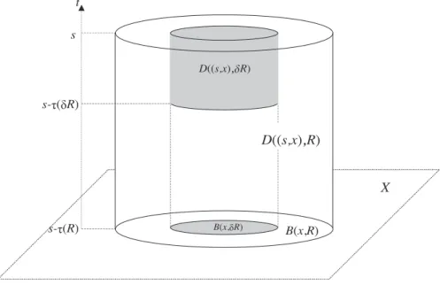
For all s2R, r >0 and x2X, define the cylinder D((s, x), r) := (s ⌧(r), s)⇥B(x, r).
For any set A⇢R⇥X and a function f on A, define ess sup
A
f = sup
t
ess sup
{x:(t,x)2A}
f(t, x), and define ess inf
A f analogously. Set
oscA f : =ess sup
A
f ess inf
A f.
4.2.1 Oscillation inequality and the H¨older continuity
Proposition 4.1 Assume that VD and LLE(⌧;") hold. Then, for any bounded caloric function u in a cylinderD((s, x), R), the following inequality holds
D((s,x), R)osc u✓ osc
D((s,x),R) u, (4.8)
(see Fig. 2), with constants , ✓ 2 (0,1) that depend only on the constants in the hypotheses.
Proof. Let m(R) and M(R) denote, respectively, the essential infimum and essential supremum of u on D((s, x), R). Since u+ const is a caloric function, we obtain by Corollary 2.3 that
u(t, y) m(R) Z
B(x,R)
pB(x,R)t ⇠ (y, z)(u(⇠, z) m(R))µ(dz), (4.9) for all s ⌧(R)< ⇠ < t < s and µ-almost all y 2B(x, R). Choose here
⇠ =s ⌧("R).
s
D((s,x), R)
B(x,R)
t
B(x,R) s- (R)
X s-( R)
D((s,x),R)
Figure 2: Cylinders D((x, s), R) andD((x, s), R)
By the properties of the function ⌧(·), there is a constant"0 2(0, ") such that
⌧("r) 2⌧("0r) for all r >0.
Then, for any t2(s ⌧("0R), s), we have t ⇠ ⌧("R),
t ⇠ ⌧("R) ⌧("0R) ⌧("0R).
It follows from (4.7) that, for this range of t, pB(x,R)t ⇠ (y, z) c1
V(x, R) for all µ-a.a. y, z 2B(x, ""0R). (4.10) Set = ""0 so that both (4.10) and (4.9) are satisfied for (t, y) 2 D((s, x), R).
Restricting the integration in (4.9) toB(x, R), using (4.10), and taking the essential infimum in (t, y)2D((s, x), R), we obtain
m( R) m(R) c1
V(x, R) Z
B(x, R)
(u(⇠, z) m(R))µ(dz). (4.11) By a similar argument using M(R) u(t, y), we obtain
M(R) M( R) c1
V(x, R) Z
B(x, R)
(M(R) u(⇠, z))µ(dz), (4.12) which together with (4.11) implies
M(R) m(R) (M( R) m( R)) c1V(x, R)
V(x, R) (M(R) m(R)) c2(M(R) m(R)),
where VD has been used in the last inequality. Rearranging this inequality, we obtain
(1 c2)(M(R) m(R)) M( R) m( R), which proves (4.8) with✓ = 1 c2.
From the oscillation inequality, a standard argument gives the H¨older continuity of caloric functions as follows.
Corollary 4.2 Assume thatVDandLLE(⌧;")hold. Then, for any bounded caloric function u in a cylinder D((t0, x0), R), the following inequality is satisfied
|u(s0, x0) u(s00, x00)| C
✓⌧ 1(|s0 s00|) +d(x0, x00) R
◆↵
D((tosc0,x0),R)u (4.13) for all almost all(s0, x0),(s00, x00)2D((t0, x0), R), where ↵, 2(0,1)andC > 0are constants that depend on the constants in hypotheses VD and LLE(⌧;").
Proof. We will prove the following equivalent form of (4.13): for any r >0 and for almost all (s0, x0),(s00, x00)2D((t0, x0), R) such that
⌧ 1(|s0 s00|) +d(x0, x00)< r, (4.14) the following inequality holds:
|u(s0, x0) u(s00, x00)| C⇣r R
⌘↵
D((tosc0,x0),R)u. (4.15) It suffices to show that any two points (s0, x0),(s00, x00)2D((t0, x0), R) with condi- tion (4.14) are contained in an open subset ⌦⇢D((t0, x0), R) such that
osc⌦ uC⇣r R
⌘↵
D((tosc0,x0),R)u. (4.16) Since the metric space (R⇥X)2is separable, the setSof couples ((s0, x0),(s00, x00)) in D((t0, x0), R)⇥D((t0, x0), R) satisfying (4.14) can be then covered by a countable family of sets like ⌦⇥⌦ where ⌦ is as above. Because in each ⌦⇥⌦ the estimate (4.15) holds almost everywhere, it follows that (4.15) holds almost everywhere inS.
Assuming thats0 s00, set y=x0 and choose t to be a bit larger than s0 so that s0 < t < t0 and
⌧ 1(t s) +d(x, y)< r (4.17)
for both the points (s, x) = (s0, x0) and (s, x) = (s00, x00) (the strict inequality in (4.14) provides a flexibility for makingtstrictly larger than s0). Then define the set
⌦ by
⌦ = D((t, y), r)\D((t0, x0), R). By construction, we have (t, y)2D((t0, x0), R), that is,
t0 ⌧( R)< t < t0 and d(x0, y)< R.
Also, it follows from (4.17) that both the points (s0, x0) and (s00, x00) belong to D((t, y), r).
Consider first the case whenD((t, y), r) is not contained inD((t0, x0), R). Then we have
d(x0, y) +r > R or t0 ⌧(R)> t ⌧(r), which implies that
r >(1 )R or ⌧(r)> ⌧(R) ⌧( R) ⌧( R)
whence it follows in the both cases r R. (Here we may and will assume that
< 1/2.) Clearly, in this case (4.16) is trivial for any ↵ > 0 just by taking the constant C larger than ↵.
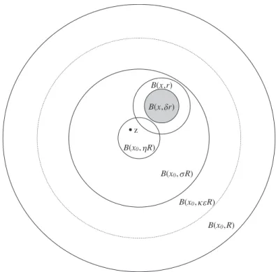
Assume now that D((t, y), r) ⇢ D((t0, x0), R), and let k 1 be a possibly large integer (to be specified below) such that
D (t, y), kr ⇢D((t0, x0), R) (4.18) (see Fig. 3).
t0
D((t0,x0), R)
t
t0- (R) t0- ( R)
D((t0,x0)
,
R)D((t,y), -kr) (t0,x0)
(t,y)
t
t- ( kr)
Figure 3: CylinderD (t, y), kr
Then by Proposition 4.1, we have
D((t,y),r)osc u✓k osc
D((t,y), kr)u✓k osc
D((t0,x0),R)u. (4.19) The value of k in (4.18) can be estimated as follows. The condition (4.18) means that
t0 ⌧(R)t ⌧ kr and d(x0, y) + kr R,
which will follow from
⌧( R) +⌧ kr ⌧(R) and R+ krR. (4.20) The value of can be assumed to be so small that
⌧( R) 1
2⌧(R) and <1/2,
so that both the conditions in (4.20) will follow from kr R. Hence, (4.18) and a forteriori (4.19) hold with
k=
log (R/r)
log (1/ ) 1 log (R/r) log (1/ ) 2.
It follows from (4.19) that
D((t,y),r)osc uC⇣r R
⌘↵
D((tosc0,x0),R)u, (4.21) where↵ = log(1/✓)log(1/ ) and C =✓ 2.
Remark. It follows from Corollary 4.2 that any locally bounded caloric function u(t, x), defined in a cylinder, is continuous in its entire domain; more precisely, it has a version that is jointly continuous in (t, x). Hence, in the rest of the proof of (b))(c) we can assume that all locally bounded solutions are continuous.
4.2.2 Obtaining the Harnack inequality
We can now complete the proof of (b))(c). It follows from (3.1) that there exists a (small) constant l2(0,1) such that
⌧(r) 2⌧(lr) (4.22)
for all r > 0. We will prove w-PHI(⌧) in a slightly di↵erent, but equivalent form:
if u(t, x) is a bounded (and hence continuous) non-negative caloric function in the cylinder
Q= (0, ⌧ ("R))⇥B(x0, R),
wherex0 2X and R >0 are arbitrary and" is the parameter from LLE(⌧;"), then sup
Q
uCinf
Q+
u, where
Q = (⌧(l3"R), ⌧(l2"R))⇥B(x0, ⌘R), Q+ = (⌧(l"R), ⌧("R))⇥B(x0, ⌘R), (4.23) and the constants⌘2(0,1), C > 1 depend only on the constants in the hypotheses.
It is enough to show that if infQ+u1 then supQ uC.
The essential part of the proof is contained in the following claim.
Claim. Let (t, x)2Q and r >0 be such that
D((t, x), r)⇢Qe:= (0, ⌧(l2"R))⇥B(x0, R) (4.24) where is a constant to be specified later on; so far let us assume ⌘ < < 1 (see Fig. 4). If
u(t, x) , then
sup
D((t,x),r)
u K ,
with some constant K >1, provided satisfies the inequality C
✓R r
◆
, (4.25)
where is the constant from (3.11) andCis a large enough constant. Both constants C and K depend only upon the constants in the hypotheses.
( R)
Q+
B(x0, R)
0 B(x0,R)
(l R)
(l2 R)
(l3 R)
X B(x0, R)
Q- (T,z) Q
(t,x)
D((t,x),r) Q~
Figure 4: CylinderD((t, x), r)
Observe first that, by Corollary 2.3, we have, for allt < T < ⌧("R) andµ-almost all z 2B(x0, R), that
u(T, z) Z
B(x0,R)
pB(xT t0,R)(z, y)u(t, y)µ(dy). (4.26) Restrict T to the interval ⌧(l"R) < T < ⌧("R). For any 0< t < ⌧(l2"R), it follows that
⌧(R)< T t < ⌧("R), (4.27)
where = l2!, which is true by (4.22). Applying (4.7) with r = R, (4.27), and VD, we obtain
pB(xT t0,R)(z, y) c1
V (x0, R), (4.28)
for almost all z, y 2B(x0, "R). We can assume that the constant from (4.24) is so small that
". (4.29)
Then (4.28) holds for almost all z, y 2B(x0, R) (see Fig. 5).
B(x,r)
B(x0, R)
B(x0, R)
B(x0, R) B(x0,R) z
B(x, r)
Figure 5: Estimating the function u(t, y) in the ball B(x, r)
Reducing the domain of integration in (4.26) to the ball B(x, r)⇢ B(x0, R) (where <1 is the constant from Proposition 4.1) and using (4.28), we obtain, for all T as above and almost all z 2B(x0, R),
u(T, z) c1
V(x0, R) Z
B(x, r)
u(t, y)µ(dy).
In particular, this inequality holds for almost all (T, z)2Q+. Since the right hand side does not depend on T, z, taking the essential infimum in (T, z)2Q+ and using ess inf
Q+
u= infQ+u1, we obtain
1 c1
V(x0, R) Z
B(x, r)
u(t, y)µ(dy), whence
y2B(x, r)inf u(t, y)⇤ := V (x0, R) c1V (x, r).
Combining with the hypothesis u(t, x) , we see that
D((t,x), r)osc u ⇤, whence by Proposition 4.1
sup
D((t,x),r)
u osc
D((t,x),r)u ✓ 1( ⇤),
where 0< ✓ <1 is the constant from Proposition 4.1. We are left to make sure that
✓ 1( ⇤) K ,
with a constantK >1. Observe that by (3.11)
⇤C1
✓R r
◆ ,
whereC1 =C1(c1, CVD, , ). Assuming from the beginning that 2C1
1 ✓
✓R r
◆ , we obtain that ⇤ 12✓ and, hence,
✓ 1( ⇤) ✓ 1+ 1
2 ,
so that we can set K = ✓ 12+1 >1. This completes the proof of the Claim.
We can reformulate the Claim as follows. Define a function
⇢( ) = R (C )1/
so that the condition (4.25) is equivalent to r ⇢( ). If for some point (s, y)2Q, we have :=u(s, y)>0 and
D((s, y), ⇢( ))⇢Q,e
then there is a point (s0, y0)2D((s, y), ⇢( )) such that u(s0, y0) K .
Start with an arbitrary point (s0, y0)2Q where 0 :=u(s0, y0)>0. Assuming that
D((s0, y0), ⇢( 0))⇢Q,e choose a point (s1, y1)2D((s0, y0), ⇢( 0)) where
1 :=u(s1, y1) K 0. If
D((s1, y1), ⇢( 1))⇢Q,e
then select a point (s2, y2)2D((s1, y1), ⇢( 1)) such that
2 :=u(s2, y2) K 1 K2 0,
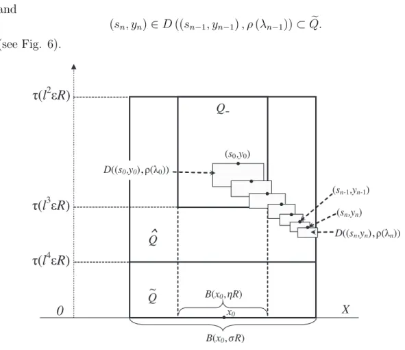
and so on. We obtain in this manner a sequence of points {(sn, yn)} such that
n :=u(sn, yn) Kn 0 and
(sn, yn)2D((sn 1, yn 1), ⇢( n 1))⇢Q.e (see Fig. 6).
Q~ Q
^
(l
2R)
B(x0, R)
0 (l
3R)
(l
4R)
X
B(x0, R)
Q-
(s0,y0) D((s0,y0), ( 0))
(sn-1,yn-1) (sn,yn)
D((sn,yn), ( n))
x0
Figure 6: The sequence of cylindersD((sk, yk), ⇢( k)) Let us continue this construction until
D((sn, yn), ⇢( n))6⇢Qb := [⌧(l4"R), ⌧(l2"R)]⇥B(x0, R). (4.30) If such n does not exist then we obtain an infinite sequence (sn, yn) 2 Qb such that u(sn, yn)! 1 which is not possible because the function u is bounded in Q.b Hence, there exists ann that satisfies (4.30). It follows that either yn2/ B(x0, R) orsn⌧(l4"R).In the former case, we have
d(y0, yn) d(x0, yn) d(x0, y0) ( ⌘)R, and in the latter case
s0 sn ⌧(l3"R) ⌧(l4"R) ⌧(R)
where=l4".
On the other hand, we have d(y0, yn)
n 1
X
k=0
d(yk, yk+1)
n 1
X
k=0
⇢( k)
n 1
X
k=0
⇢ Kk 0 C2R 01/
and similarly
s0 sn= Xn
k=0
(sk sk+1) Xn
k=0
⌧(⇢( k))⌧(C3R 01/ ),
where we have used (3.1). Comparing with the above lower bounds ofd(y0, yn) and s0 sn, we obtain in the both cases that
0 C4 =C4(C2, C3, , ⌘, ).
Since 0 is the value of uat an arbitrary point in Q , it follows that supQ uC4, which finishes the proof of w-PHI(⌧).
4.3 Proof of (c) ) (a) (w-PHI implies w-HKE)
We prove here that VD + w-PHI(⌧) implies w-HKE(⌧).
4.3.1 A technical lemma We start with the following lemma.
Lemma 4.3 For any ⌫ 2 (0,1) there exist constants , ! 2 (0,1) depending on ⌫ and on 1 from (3.1) with the following property: for anyR > 0there isr2[!R, R]
such that
⌧(r) ⌧(⌫r) ⌧(R). (4.31)
Proof. Consider sequence ri = ⌫iR, i = 0,1,2, ... and assume that, for some positive integer n, none of the values r0, ..., rn 1 satisfies (4.31), that is,
⌧(r0) ⌧(r1) < ⌧(R)
⌧(r1) ⌧(r2) < ⌧(R) ...
⌧(rn 1) ⌧(rn) < ⌧(R). Adding up all these inequalities yields
⌧(R) ⌧(rn)< n⌧(R). By (3.1) we have
⌧(R)C 1⌧(R)
and
⌧(rn) =⌧(⌫nR)C⌫n 1⌧(R) whence
⌧(R)C⌫n 1⌧(R) +nC 2⌧(R). (4.32) Choose now n =n( 1, ⌫) so big that C⌫n 1 < 12 and then choose = ( 1, ⌫) >0 so small thatnC 2 < 12. With these values ofn and equation (4.32) cannot hold, which means that there isi < n such that
⌧(ri) ⌧(ri+1) ⌧(R). Clearly, we have
ri =⌫iR ⌫nR =!R where! :=⌫n,which finishes the proof.
4.3.2 Oscillation inequality and the H¨older continuity The next statement is an analogue of Proposition 4.1.
Proposition 4.4 Assume that w-PHI(⌧) holds. Then, for any bounded caloric functionu in a cylinder D((s, x), R), the oscillation inequality (4.8) holds with con- stants , ✓ 2(0,1) that depend only on the constants in the hypotheses.
Proof. Fix some r >0 and consider the cylinders
Q(r) :=Q(x, ⌧(C4r), C5r) = (0, ⌧(C4r))⇥B(x, C5r) and
Q (r) := (⌧(C1r), ⌧(C2r))⇥B(x, r), Q+(r) := (⌧(C3r), ⌧(C4r))⇥B(x, r),
as in the definition of w-PHI(⌧). We would like to choose r such that Q(r)⇢D((s, x), R) = (s ⌧(R), s)⇥B(x, R) and
Q+(r) D((s, x), R) = (s ⌧( R), s)⇥B(x, R) (see Fig. 7).
The inclusions of the corresponding balls occur if
R C5r and r R. (4.33)
To handle the inclusion of the time intervals, first make a shift of time to ensure s=⌧(C4r). Then the inclusions of the time interval occur provided
⌧(R) ⌧(C4r) and ⌧( R)⌧(C4r) ⌧(C3r). (4.34)
s= (C4r) t
s- (R) (C2r)
D((s,x),R)
(s,x)
(C3r)
(C1r)
Q(r)
Q-(r)Q+(r)
D((s,x), R)
0 s- ( R)
Figure 7: Cylinders Q(r), Q+(r), Q (r)
Setting ⌫ = CC3
4 and R0 = R/C5, observe that by Lemma 4.3 there exists r0 2 [!R0, R0] such that
⌧(r0) ⌧(⌫r0) ⌧(R0),
where and ! are positive constants depending on ⌫ and 1. Setting r=r0/C4 we obtain that
!RC4C5r R and ⌧(C4r) ⌧(C3r) ⌧ C51R so that both the conditions (4.33) and (4.34) are satisfied with
= min
✓ ! C4C5
, C5
◆ .
Let m(R) and M(R) be the essential infimum and essential supremum of u on D((s, x), R). Applying w-PHI(⌧) to the function u m(R) in Q(r), we obtain
ess sup
Q (r)
(u m(R)) C6 ess inf
Q+(r) (u m(R))
C6 ess inf
D((s,x), R)(u m(R))
= C6(m( R) m(R)), and in the same way
ess sup
Q (r)
(M(R) u)C6(M(R) M( R)).
Adding up the two inequalities, we obtain M(R) m(R) ess sup
Q (r)
((M(R) u)+ ess sup
Q (r)
(u m(R))
C6(m( R) m(R)) +C6(M(R) M( R)), whence
M( R) m( R)(1 1
C6
)(M(R) m(R)).
Hence, (4.8) holds with ✓= (1 1/C6).
Corollary 4.5 Assume thatw-PHI(⌧) holds. Then the conclusion of Corollary 4.2 holds. In particular, any locally bounded caloric function has a continuous version.
The proof is the same as that of Corollary 4.2. In what follows we will always use the continuous versions of locally bounded solutions.
4.3.3 Existence of the heat kernel and on-diagonal upper bound
We next show the existence and an on-diagonal upper bound of the heat kernel under the assumption w-PHI(⌧). Letf be a non-negative function fromf 2L2\L1(X, µ).
The functionv(t, x) = etLf(x) is a non-negative essentially bounded caloric function in R+⇥X. By the previous section, this function has a continuous version; let us denote in the sequel by Ptf(x) the continuous version ofetLf.
Choose somer >0,x2X, setB =B(x, r) andtk =⌧(Ckr) wherek = 1,2,3,4 and Ck are the constants from w-PHI(⌧). Applying the Harnack inequality in the cylinderQ(x, ⌧(C4r), C5r), we obtain, for any t 2(t1, t2),
Ptf(x)C6 inf
t3<s<t4,y2BPsf(y). (4.35) Since kPsfk2 kfk2, it follows that
t3<s<tinf4,y2B(Psf(y))2 1 (t4 t3)µ(B)
Z t4
t3
Z
B
(Psf(y))2dµ(y)ds kfk22
V (x, r). Setting in (4.35)t =⌧ C1+C2 2r and noticing thatr =c⌧ 1(t), where
c= 2
C1+C2
, we obtain that, for allt >0 and x2X,
Ptf(x) Ckfk2
V (x, c⌧ 1(t))1/2, (4.36)
whereC =C6.
Let us extend (4.36) to all non-negative functions f 2 L2(X). Indeed, setting fn := min (f, n) we obtain fn 2 L2 \L1 so that (4.36) holds for fn. Hence, the