RIMS-1773
Fluctuations of recentered maxima of discrete Gaussian Free Fields on a class of recurrent graphs
By
Takashi KUMAGAI and Ofer ZEITOUNI
February 2013
R ESEARCH I NSTITUTE FOR M ATHEMATICAL S CIENCES
Fluctuations of recentered maxima of discrete Gaussian Free Fields on a class of recurrent graphs
Takashi Kumagai
⇤Ofer Zeitouni
†February 8, 2013
Abstract
We provide conditions that ensure that the recentered maximum of the Gaussian free field on a sequence of graphs fluctuates at the same order as the field at the point of maximal variance. In particular, on a sequence of such graphs the recentered maximum is not tight, similarly to the situation inZbut in contrast with the situation inZ2. We show that our conditions cover a large class of “fractal” graphs.
1 Introduction
The study of the maxima of Gaussian fields has a rich history, which we will not attempt to survey here. The general theory was developed in the 70s and 80s, and an excellent account can be found in [18]. However, general results concerning the order of fluctuations of the maximum are lacking.
In recent years, a special e↵ort has been directed toward the study of the so called Gaussian free field (GFF) on various graphs. While we postpone the general definition to the next section, we discuss in this introduction the special case of the GFF on subsets VN = ([ N, N]\Z)d, with Dirichlet boundary conditions. These are random fields{Xx}x2VN
indexed by points inVN, with joint density (with respect to Lebesgue measure) proportional to
exp cX
x⇠y
(Xx Xy)2
! ,
with the sum over neighbors in VN, and Xx = 0 for x 2 @VN. (An alternative description involving the Green function of random walk onVN is given below in Section 2; see also [20]
⇤Research partially supported by the Grant-in-Aid for Scientific Research (B) 22340017.
†Research partially supported by NSF grant #DMS-1106627 and a grant from the Israel Science Foun- dation.
for a very readable introduction to GFFs in a continuous setting.) With XN,d⇤ denoting the maximum of the GFF onVN in dimensiond, it is not hard to see thatXN,d⇤ is of orderp
N for d= 1, order logN for d= 2, and order (logN)1/2 ford 3. Moreover, a consequence of the Borell-Tsirelson inequality (see [18]) is that ford 3, since simple random walk is transient on Zd, the fluctuations of XN,d⇤ are at most of order 1, while for d = 1 the fluctuations of XN,1⇤ are of the same order as XN,1⇤ , i.e. of order p
N. The critical case d = 2 was settled only recently [8], where it was shown that the fluctuations of XN,2⇤ are also of order 1. This raises naturally the question of determining for which sequences of graphs is the sequence of recentered maxima of the GFF tight.
Our goal in this paper is to exhibit a class of sequences of graphs, which are fractal-like and for which the maximum of the GFF fluctuates at the same order as the maximum itself, and both are of the order of the maximal standard deviation of the GFF in the graph. In that respect, the behavior of the maximum is similar to that ofXN,1⇤ . For this class of graphs, we also show that thecover time of the graph, measured in terms of the (square root of the) local time at a fixed vertex, also does not concentrate. (We note in passing that for the cover time ofVN in two dimensions, it is, to the best of our knowledge, an open problem to decide whether this quantity concentrates or not.)
The structure of the paper is as follows. In the next section, we introduce the GFF on general graphs and state Assumption 2.1 that characterizes the graphs which we investigate;
the main feature is a relation between the graph distance and the resistance, and control of the covering number of the graph in terms of resistance distance. We then state our main result, Theorem 2.2, concerning fluctuations of the maximum of the GFF. We also state Proposition 2.4 concerning the cover time of the graphs. Proofs of the theorem and proposition are given in Section 3. The heart of the paper is then Section 4.1, where we show that certain naturally constructed fractal-like graphs satisfy our assumptions. In particular, this is the case for the standard Sierpinski carpets in two dimensions and gaskets in all dimensions.
Notation Throughout the paper, we usec1, c2,· · · to denote generic constants, indepen- dent ofN, whose exact values are not important and may change from line to line. We write an ⇣bn if there exist constants c1, c2 >0 such that c1bnan c2bn for all n 2N.
2 Framework
We first introduce general notation for finite graphs with a ‘wired’ boundary and their associated resistance. Let G= (V(G), E(G)) be a connected (undirected) finite graph with at least two vertices, where V(G) denotes the vertex set andE(G) the edge set ofG. LetdG
be the graph distance, that is,dG(x, y) is the number of edges in the shortest path fromxto
y in G. Define a symmetric weight function µG :V(G)⇥V(G)!R+ that satisfies µGxy >0 if and only if {x, y}2E(G). For B ⇢G with B 6=G and for distinctx, y 2V(G) not both inB, we define theresistance betweenx and y by
RB(x, y) 1 := inf{1 2
X
w,z2V(G)
(f(w) f(z))2µGwz :f(x) = 1, f(y) = 0, f|B = constant}. We set RB(x, x) = 0, RB(x, y) = 0 if x, y 2B and, for x2V(G)\B, we define RB(x, B) = RB(x, y) for any y2B. We write R(x, y) := R;(x, y).
The resistance RB(·,·) is the resistance of the following electrical network with a ‘wired’
boundary: Consider the graph Gobtained by combining all vertices in B to a single vertex b, that is V(G) = (V(G)\B)[{b} and
E(G) = {{x, y}:{x, y}2E(G), x, y 2G\B}
[{{x, b}:x2G\B, 9y2Bwith{x, y}2E(G)}. Define the modified symmetric weight function
µGxy =
( µGxy, x2V(G)\ {b}, y 2V(G)\ {b}, P
z2BµGxz, x2V(G)\ {b}, y =b , and set as before µGx =P
y2V(G)µGxy. Let {wt}t 0 be the continuous time random walk on G such that the holding time at a vertex is exp(1), and the jump probability is given by µx,y/µx. Let
Lx,Nt = 1 µGx
Z t 0
1{ws=x}ds
denote the (weight normalized) local time at x.
Now, let {GN}N 1 be a sequence of finite connected graphs such that |GN| 2 for all N 1 and limN!1|GN|=1. For eachGN = (V(GN), E(GN)), we take a symmetric weight functionµGN, a boundaryBN ⇢GN withBN 6=GN, and the corresponding continuous time Markov chain{wNt }t 0 with the wired boundary condition onBN as above. We assume that GN \BN is connected. Let TN := min{t 0 : wNt = b}, and define, for each x, y 2 V(GN)\BN, GN(x, y) =EGxN[Ly,NTN] where EGxN denotes the expectation with respect to wNt started at x. For z 2BN, we set XzN ⌘0. The Gaussian free field (GFF for short) on GN (with boundary BN) is the zero-mean Gaussian field {XzN}z2V(GN) with covariance GN(·,·).
It can be easily checked (using for instance [9, Lemma 2.1], [15, Proposition 3.6]) that E[(XxN XyN)2] =RBN(x, y).
Let h : N ! N be a strictly increasing function with h(0) = 0, that satisfies the following doubling property: there exist 0< 1 2 <1andC >0 such that, for all 0< rR <1,
C 1
✓R r
◆ 1
h(R) h(r) C
✓R r
◆ 2
. (2.1)
We assume the following.
Assumption 2.1. There exist ↵ > 0 and c1, c2, c3 > 0 such that the following hold for all large N.
(i) RBN(x, y)c1h(dGN(x, y)) for all x, y 2GN.
(ii) maxx2GNRBN(x, BN) c2maxx2GNh(dGN(x, BN)) for all x2GN.
(iii) NGN( dNmax)c3 ↵ for all 2(0,1] where dNmax := maxx2GNdGN(x, BN)and NGN(") is the minimal number of dGN-balls of radius" needed to coverGN. Furthermore,dNmax ! 1 as N ! 1.
LetXN⇤ = maxz2V(GN)XzN and define ˜XN =XN⇤/ N, where N = (maxz2GNE[(XzN)2])1/2. Note that 2N = maxx2GNRBN(x, BN), and limN!1 N =1 under Assumption 2.1(iii).
Theorem 2.2. Under Assumption 2.1, there exist constants A, B, A0 > 0 and a function g : (0,1)!(0,1) such that the following holds for all N large.
P( ˜XN < A)> B, P( ˜XN > c) g(c) 8c >0, E( ˜XN)A0. (2.2) In particular, under Assumption 2.1, {XN⇤ EXN⇤}N fluctuates with order N and there- fore it is not tight.
Remark 2.3. We stated Assumption 2.1 with respect to the graph distance in GN, because this will be easiest to check in the applications. However, one should note that the proof of Theorem 2.1 does not depend on the particular metric chosen, as long as the metric satisfies the assumption. In particular, if we choose RBN(·,·) as the metric, Assumption 2.1 (i), (ii) turns out to be trivial with h(s) = s, and the assumption boils down to NRBN( 2N)c3 ↵
for all 2(0,1] and limN!1 N =1, where NRBN(") is the minimal number of RBN-balls of radius " needed to cover GN.
In a recent seminal work, [9] have established a close relation between the expectation of the maximum of the GFF on general graphs and the expected cover time of these graphs by random walk. Under the assumptions of Theorem 2.2, one can also derive information on the fluctuations of the cover time, as follows. Define the cover time of GN as
⌧cov = infN {t >0 :Lx,Nt >0, 8x2GN}. It is easy to see
⌧cov = inf{N t >0 :8x2GN,9st such that wNs =x}.
We will consider the square-root of the normalized local time at BN at cover time, i.e. the random variable LN := q
Lb,N⌧N
cov. One expects (see [9]) that LN should behave similarly to |XN⇤|. In the special case of GN being the rooted at b binary tree of depth N, this was confirmed in [7]. In our setup here, this is confirmed in the following proposition.
Proposition 2.4. With notation as above and under Assumption 2.1, the conclusion of Theorem 2.2 hold with LN/ N replacing X˜N.
3 Proofs of Theorem 2.2 and Proposition 2.4
We begin with the proof of Theorem 2.2.
Proof of Theorem 2.2: Let ˜d(x, y) = (E[(XxN XyN)2])1/2/ N = RBN(x, y)1/2/ N. Then, using Assumption 2.1 (i),(ii), there exists c >0 such that for allx, y 2GN withdGN(x, y) dNmax and allN 2N,
d(x, y) =˜ ⇣RBN(x, y)
2N
⌘1/2
c⇣h(dGN(x, y)) h(dNmax)
⌘1/2
cC⇣dGN(x, y) dNmax
⌘ 1/2
.
Thus, denoting Nd˜(") the minimal number of ˜d-balls of radius " needed to cover GN, we have
Nd˜(cC 1/2)NGN( dNmax)c3 ↵,
where we used Assumption 2.1 (iii) in the second inequality. Rewriting this, we haveNd˜(") c0" 2↵/ 1, wherec0 >0 is independent of N. Set = 2↵/ 1. We can apply [1, Theorem 5.2]
to deduce that there exist 0 >0 and N0 such that for all > 0, ">0 and N > N0, P( ˜XN > )C +1+" ( ),
where C 1 does not depend on N and ( ) = (2⇡) 1/2R1
e x2/2dx. On the other hand, letx⇤N be such that E(Xx2⇤
N) = 2N. Then, for any >0, P( ˜XN > ) P(XxN⇤
N > N) = ( ).
The estimates in (2.2) are easy consequences of the last two displayed inequalities. 2 We turn to the analysis of cover times.
Proof of Proposition 2.4: The upper bound in the proposition is a consequence of the Eisenbaum-Kaspi-Marcus-Rosen-Shi isomorphism theorem [10], as was observed in [9]: in- deed, by [9, Eq. (20),(21)] and using the last estimate in (2.2), there exist constantsc1, c2 >0 so that with t=✓ 2N, and all ✓ large enough,
P(min
x Lx,N⌧N(t) t/2)c1e c2✓ (3.1) while
P(max
x Lx,N⌧N(t) 2t)c1e c2✓, (3.2) where ⌧N(t) := inf{s >0 :Lb,Ns > t}.
On the event {minxLx,N⌧N(t) t/2}we have that ⌧N(t) ⌧cov. Thus, on the eventN {min
x Lx,N⌧N(t) t/2}\{max
x Lx,N⌧N(t) 2t}, one has that
Lb,N⌧N
cov Lb,N⌧N(t) max
x Lx,N⌧N(t) 2t . (3.3) In particular, (3.1), (3.2) and (3.3) imply that ELN/ N is bounded uniformly.
To estimate LN from below, we use the Markov property. Let x⇤ 2 V(GN) be such that RBN(x⇤, BN) = 2N and let Tx⇤ = inf{t : wNt = x⇤}. Since ⌧covN Tx⇤, we have that
LN q
Lb,NTx⇤. We decompose the walk wNt according to excursions from b: the probability to hit x⇤ during one excursion (see e.g. [19, Ch. 2]) is
pN = 1
2NµN
,
where µN =µGbN .Therefore,
Lb,NTx⇤ =d 1 µN
ZN
X
i=1
Ei,
whereZN is geometric of parameterpN andEiare standard independent exponential random variables. Note that ELb,NTx⇤ = 2N.
Consider now a parameter ⇠>0. We have that P(Lb,NTx⇤ ⇠ 2N) P(ZN ⇠/pN)P
0
@ 1 µN
⇠/pN
X
i=1
Ei >⇠ 2N 1 A
P(ZN ⇠/pN)P 0
@pN
⇠
⇠/pXN
i=1
Ei 1 1
A=:P1P2.
Note that from the properties of the geometric distribution, regardless of pN we have that P1 c1(⇠) >0. On the other hand, if pN ! 0 then pNP1/pN
i=1 Ei ! 1 a.s., and in any case we also have that P2 c2(⇠)>0. We conclude that
P(LN p
⇠ N) c1(⇠)c2(⇠).
2
4 Examples
4.1 Nested fractal graphs and strongly recurrent Sierpinski carpet graphs
Let { i}Ki=1 be a family of L-similitudes on Rd for some L > 1, that is, for each i, i is a map from Rd to Rd such that i(x) = L 1Uix+ i, x 2 Rd, where Ui is a unitary map and i 2 Rd. We assume that { i}Ki=1 satisfies the open set condition, namely there exists a non-empty bounded set O ⇢ Rd such that { i(O)}Ki=1 are disjoint and [Ki=1 i(O) ⇢ O.
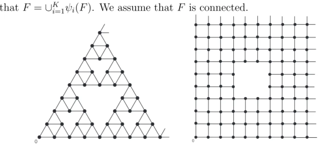
Since { i}Ki=1 is a family of contraction maps, there exists a unique non-empty compact set F such thatF =[Ki=1 i(F). We assume that F is connected.
0 0
Fig 1: 2-dimensional Sierpinski gasket graph and carpet graph 4.1.1 Nested fractal graphs
Let⌅ be the set of fixed points of { i}Ki=1, and define
V0 :={x2⌅: 9i, j 2{1, . . . , K},i6=j and y2⌅ such that i(x) = j(y)}.
Assume that #V0 2 and set i1...in := i1 · · · in. F is then called a nested fractal if the following holds.
• (Nesting) If i1. . . in and j1. . . jn are distinct sequences in {1, . . . , K}, then
i1...in(F)\ j1...jn(F) = i1...in(V0)\ j1...jn(V0).
• (Symmetry) If x, y 2 V0, then the reflection in the hyperplane Hxy := {z 2 Rd :
|z x|=|z y|} maps SK
i1,...,in=1 i1...in(V0) to itself.
We assume without loss of generality that 1(x) =L 1x and that the origin belongs to V0. Let
V(GN) :=
[K i1,...,iN=1
LN i1...iN(V0), G:=
[1 N=1
V(GN). (4.1)
Next, define B0 := {{x, y} : x 6= y 2 V0}. Then inside each LN i1...iN(V0), N 0,1 i1,· · · , iN K, we place a copy of B0 and denote byB the set of all the edges determined in this way. Next, we assign µxy = µyx > 0 for each {x, y} 2 B in such a way that there exist c1, c2 >0 such that
c1 µxy =µyxc2, 8{x, y}2B.
We call the graph (G, µ) a nested fractal graph. A typical example is the 2-dimensional Sierpinski gasket graph in Fig 1 (whereL= 2). Letd(·,·) be the graph distance onG,{wk}k the Markov chain for (X, µ), and define the heat kernel aspk(x, y) = Px(wk =y)/µy. (Note that we consider the discrete time Markov chain here in order to apply the results in [5] to derive the resistance estimates (4.5). Indeed, (4.5) can be obtained through both discrete and continuous time Markov chains.) It is known (see [12] (also [16] for the continuous setting)) that there exist constants c3, . . . , c6 such that for all x, y 2G, k >0
pk(x, y)c3k df/dwexp c4
✓d(x, y)dw k
◆1/(dw 1)!
, (4.2)
and for k > d(x, y),
pk(x, y) +pk+1(x, y) c5k df/dwexp c6
✓d(x, y)dw k
◆1/(dw 1)!
, (4.3)
where dw = log(⇢K)/log(L⌘), df = logK/log(L⌘) with some constants ⇢ >1, ⌘ 1. df is called theHausdor↵ dimension and dw is called the walk dimension. For the 2-dimensional Sierpinski gasket graph, L= 2,⌘= 1, K = 3 and⇢= 5/3. Noting that dw > df and that
c7Rdf µ(B(x, R))c8Rdf, 8x2G, R 1, (4.4) (4.2), (4.3) implies (see [5, Theorem 1.3, Lemma 2.4])
R(x, y)c9d(x, y)dw df, R(x, Bc(x, R)) c10Rdw df, 8x, y 2G, 8R 1. (4.5) We now define a sequence of graphs {GN}N 0 by setting V(GN) as above and E(GN) :=
{{x, y} 2 B : x, y 2 V(GN)}. Let dGN(·,·) be the graph distance on GN; one can easily see that d(x, y) dGN(x, y) for x, y 2 GN. (Note that |x y| ⇣ dGN(x, y)logL/log(L⌘) for x, y 2GN (cf. [16, Section 3]) and logL/log(L⌘) is called the chemical-distance exponent.) Let BN :=LNV0. Clearly RBN(x, y) R(x, y) for x, y 2 GN and dNmax ⇣ dGN(0, BN)⇣ (L⌘)N. So (4.5) implies Assumption 2.1 (i),(ii) with h(s) =sdw df, and (4.4) with the self- similarity of the graph imply Assumption 2.1 (iii) with↵=df. We note that we can actually take BN arbitrary as long as dNmax ⇣(L⌘)N.
4.1.2 Strongly recurrent Sierpinski carpet graphs
Let H0 = [0,1]d, and let L 2 N, L 2 be fixed. Set Q = {⇧di=1[(ki 1)/L, ki/L] : 1 ki L (1 i d)}, let L K Ld and let { i}Ki=1 be a family of L-similitudes of H0
onto some element of Q. We assume that the sets i(H0) are distinct, and as before assume
1(x) = L 1x. Set H1 = [Ki=1 i(H0). Then, there exists a unique non-void compact set F ⇢ H0 such that F =[Ki=1 i(F). We assume F is connected. F is called a (generalized) Sierpinski carpet if the following hold (cf. [4]):
(SC1) (Symmetry) H1 is preserved by all the isometries of the unit cubeH0.
(SC2) (Non-diagonality) Let B be a cube in H0 which is the union of 2d distinct elements of Q. (So B has side length 2L 1.) Then if Int(H1\B) is non-empty, it is connected.
(SC3) (Borders included) H1 contains the line segment {x: 0x1 1, x2 =· · ·=xd= 0}. The main di↵erence from nested fractals is that Sierpinski carpets are infinitely ramified, i.e. F cannot be disconnected by removing a finite number of points.
LetV0 be a set of vertices inH0 and defineV(GN) and Gas in (4.1). SetB0 :={{x, y}: x 6= y 2 V0,|x y| = 1}, and define B and µxy as in the case of nested fractal graphs.
We call the graph (G, µ) a Sierpinski carpet graph. A typical example is the 2-dimensional Sierpinski carpet graph in Fig 1.
It is known, see [3] and also [4] for the continuous setting, that (4.2), (4.3) hold, where dw = log(⇢K)/logL, df = logK/logL with some constant ⇢ > 0. For the 2-dimensional Sierpinski gasket graph,L= 3, K = 8 and⇢>1. Let us restrict ourselves to the case ⇢>1, namelydw > df. In this case, since (4.4) holds, we can show that (4.2) and (4.3) imply (4.5) as before. Arguing further as before, we have Assumption 2.1 (i)–(iii) with h(s) = sdw df and ↵=df.
4.2 Homogeneous random Sierpinski carpet graphs
Let ` 2 and I :={1,· · · ,`}. For each k 2 I, let { ik}Ki=1k be a family of Lk-similitudes as in the definition of the Sierpinski carpet graphs. As before, we assume 1k(x) = Lk1x. For
⇠ = (k1,· · · , kn,· · ·)2I1 and n2N, write ⇠|N = (k1,· · · , kN)2IN, and let V(GN⇠|N) := [
ij2{1,···,Kkj}, 1jN
Lk1· · ·LkN
kN
iN · · · ik11(V0), G⇠:=
[1 N=1
V(GN⇠|N). (4.6)
Let B0 := {{x, y} : x 6= y 2 V0,|x y| = 1}, and define B = B⇠ as in the cases of nested fractal graphs and carpet graphs. For simplicity, put weight µxy ⌘ 1 for each {x, y} 2 B.
We call the graph (G⇠, µ⇠) a homogeneous (random) Sierpinski carpet graph.
Fixn 2N,⇠|n= (k1,· · · , kn)2In, and letBn =Lk1· · ·Lkn,Mn =Kk1· · ·Kkn. We write Rn for the e↵ective resistance between{0}⇥[0, Bn]d 1\Gn⇠|n and {Bn}⇥[0, Bn]d 1\Gn⇠|n
inGn⇠|n, and define Tn =RnMn. Now set df(n) = logMn
logBn
, dw(n) = logTn
logBn
.
Forx2G⇠ and r 1, let Vd(x, r) be the number of vertices in the ball of radius r centered atx w.r.t. the graph distance. It can be easily seen that
c1rdf(n)Vd(x, r)c2rdf(n) if Bn r < Bn+1, x2G⇠. (4.7) Define a time scale function ⌧ : [1,1) ! [1,1) and resistance scale factor h : [1,1) ! [1,1) as
⌧(s) =sdw(n), h(s) = sdw(n) df(n) if Tns < Tn+1.
We set ⌧(0) =h(0) = 0. Note that ⌧ and h satisfy the property in (2.1) since ` <1. Given these, it is possible to obtain heat kernel estimates similar to those in Theorem 6.3 and Lemma 6.7 of [13] by tracking the proof in [13] faithfully (see the Appendix for a sketch). By making additional computations (similar to those in [11, Lemma 3.19]) in the proof of [13, Lemma 3.10], we can obtain the following heat kernel estimates (cf. Remark after Theorem 24.6 in [14]): There exist c3,· · · , c6 >0 such that ifk 2N, x, y 2G⇠, then
pk(x, y) c3
Vd(x,⌧ 1(k))exp⇣ c4
⌧(d(x, y)) k
1/( 1 1)⌘
, (4.8)
pk(x, y) +pk+1(x, y) c5
Vd(x,⌧ 1(k)) for k c6⌧(d(x, y)). (4.9) Now assume the following limits exist and the inequality holds.
df := lim
n!1df(n), dw := lim
n!1dw(n), dw > df. (4.10) Under this assumption, we have
c7
⌧(d(x, y))
Vd(x, d(x, y)) R(x, y)c8
⌧(d(x, y))
Vd(x, d(x, y)), 8x, y 2G⇠. (4.11) The equivalence of (4.8)+(4.9) and (4.11) is proved in [5] when ⌧(s) = s for some 2 under some volume growth condition referred as (V G( )). Here we need a generalized version of this under the doubling property of⌧. In fact, we only need (4.8)+(4.9))(4.11), and the generalization of this direction is easy. Indeed, using (4.8) and (4.9), we can obtain the scaled Poincar´e inequality and the lower bound of (4.11) similarly to the proof of [5, Proposition 4.2] (with ⌧(s) replacing s there). Under (4.10), a condition corresponding to (V G((dw) )) in [5] holds, so together with the scaled Poincar´e inequality, we can obtain the upper bound of (4.11) similarly to the proof of [5, Lemma 2.3 (b)].
Now let B⇠|N :=BNV0. ClearlyRB⇠|N(x, y)R(x, y) forx, y 2GN⇠|
N and dNmax ⇣BN. So (4.11) implies Assumption 2.1 (i),(ii), and (4.7), (4.10) with the homogeneity of the graph imply Assumption 2.1 (iii) with ↵ = maxndf(n). As before we can take B⇠|N arbitrary as long as dNmax ⇣BN.
Finally we will introduce randomness on this graph. Let (IN,F,P) be a Borel probability space where the measure P is stationary and ergodic for the shift operator ✓ : IN ! IN defined by ✓((k1,· · · , kn,· · ·)) = (k2,· · · , kn,· · ·). Then, by [13, Proposition 7.1] and the sub-additive ergodic theorem, one can prove the existence of the first two limits in (4.10).
Let dif, diw be the Hausdor↵ dimension and the walk dimension for Gi where i= (i, i, i,· · ·) fori2I. Let us consider a special case when d= 3,`= 2, andP is the Bernoulli probability measure with P(⇠1 = 1) = p, P(⇠1 = 2) = 1 p for some p 2 [0,1]. One can see that df/dw is a continuous function of p. Indeed, it can be easily seen that it is enough to prove limn!1Rn/n is continuous forp. By the proof of [13, Proposition 7.1], there existc1, c2 >0 such that we have
1
kElog(c1Rk) lim
n!1
1
nRn 1
kElog(c2Rk), P a.s.,
for any k 1 where E is the average over P. Since Elog(ciRk), i= 1,2 are continuous for p (because the graph is finite), we obtain the desired continuity of limn!1Rn/n. So, when we choose the two carpets in such a way that d1w > d1f and d2w < d2f (which is possible, see [4, Section 9]), we are able to construct a one parameter family of homogeneous random Sierpinski carpet graphs where df/dw is P-a.e. an arbitrary fixed number between d1f/d1w and d2f/d2w. In particular, there exists p⇤ 2(0,1) such that (4.10) holdsP-a.e. for all p < p⇤.
A Appendix: Heat kernel estimates for Markov chains on homogeneous random Sierpinski carpet graphs
In this appendix, we will briefly sketch the proof of (4.8) and (4.9). The Markov chain we consider here is the discrete time Markov chain.
Set Vn:=V(Gn⇠|n). We first define the Dirichlet form as follows.
En(f, g) := X
x,y2Vn {x,y}2B
(f(x) f(y))(g(x) g(y)), 8f, g :Vn!R.
Given two processes Y1, Y2, defined on the same state space, we define a coupling time of Y1 and Y2 as
TC(Y1, Y2) = inf{t 0 :Yt1 =Yt2}.
Let m n. We call sets of the form Lk1· · ·Lkn ikn mn m · · · ik11([0,1]d)\Vn m-complexes.
ForA ⇢G⇠, define
Dm0(A) = {m-complex which contains A},
Dm1(A) = Dm0(A)[{B :B is a m-complex, D0m(A)\B 6=;}.
LetSBz denote the exit time from the set B, when the process is started from the point z.
Theorem A.1. (Coupling) There exist0< p0 <1and K0 2N such that for eachx, y 2G⇠, there exist Markov chains wxt, wyt with wx0 = x, wy0 = y on G⇠ whose laws are equal to the simple random walk that satisfy the following: For n > K0 and y2Dn K0 0(x),
P(TC(wxt, wty)<min{SDx1
n(x), SDy1
n(x)})> p0.
The proof of the theorem follows in the same way as [4, Section 3], as G⇠ and wxt have enough symmetries for the argument there to work.
Once we have the coupling estimate, we can deduce the uniform (elliptic) Harnack in- equality as in [4, Section 4]. Let L be the infinitesimal generator associated with the simple random walk.
Theorem A.2. There exists c1 >0 such that for each x0 2G⇠, and each f :B(x0,2R)! [0,1) with Lf(x) = 0 for all x2B(x0,2R) = 0, R 1, it holds that
x2maxB(x0,R)f(x)c1 min
x2B(x0,R)f(x). (A.1)
We next introduce the following Poincar´e constant:
n = sup{X
x2Vn
(u(x) huiVn)2 |u:Vn !R,En(u, u) = 1}, where huiA= (]A) 1P
x2Au(x) for any finite set A and u:Vn!R.
The following proposition can be proved similarly to Proposition 3.1, Corollary 3.7 of [13] and (2.3), (4.4) of [17]. (Note that Theorem A.2 is needed in the proof of (A.3).) Proposition A.3. There exist constants c1,· · · , c4 >0 such that for each n, m2N,
c1RnR✓n⇠|m Rn+mc2RnR✓n⇠|m, (A.2)
c3 n Tnc4 n. (A.3)
Lemma A.4. There is a constant c such that ifTn 1 t Tn, then
pt(x, y)cMn1. (A.4)
Proof. From the definition of the Dirichlet form and the Poincar´e constant, the proof is
similar to [17, Theorem 3.3] by using Proposition A.3. 2
The next lemma can be proved similarly to [13, Lemma 3.8].
Lemma A.5. There exist c1, c2 >0 such that c1TrESDz1
r(x) for all z 2D0r(x), ESDz1
r(x) c2Tr for all z 2Dr1(x).
Since SD1l(x)t+ 1(SD1
l>t)(SDl1 t) we have, from Lemma A.5, c1Tl ESDz1
l t+E⇥ 1(Sz
D1 l
>t)E[SDX1t l]⇤
t+P(SDz1
l > t)c2Tl for t 0, z 2D0l(x).
Thus, we deduce the following: there existc3 >0,c4 2(0,1) such that P(SDz1
l(x) t)c3Tl 1t+c4 for t 0, z 2Dl0(x). (A.5) We can improve this to an exponential estimate on P(SDz1
l(x) t). In order to do this we define the following function of time and space,
k =k(n, l) = inf l0 n : Tl0
Bl0
Tl
Bn
. (A.6)
The next lemma corresponds to [13, Lemma 3.10]. Since the labeling here di↵ers from that in [13], we give the proof.
Lemma A.6. There exist constants c1, c2 such that if k = k(n, l) as in (A.6) then for all x2E, and n, l 0,
P(SDx1
n(x) Tl)c1exp ( c2Bn/Bk). (A.7) Proof. If l0 n, then for the simple random walk to cross one n-complex it must cross at least N =Bn/Bl0, l0-complexes. So, there exists 0< c <1 such that
SDx1 n(x)
cBXn/Bl0
i=1
Vixi,
where xi depend only on V1x1, . . . , Vixi11, and Viy have the same distribution as SDy1
l0(y). The deviation estimate [2, Lemma 1.1] states that ifP(Viy < s)p0+↵s, where p0 2(0,1) and
↵>0, then
logP XcN
1
Vixi t)2(↵c1N t/p0)1/2 c2Nlog(1/p0). (A.8) Thus, using (A.5) and (A.8), we have
logP(SDx1
n(x) Tl)c3(Bn/Bl0)1/2[(Tl/Tl0)1/2 c4(Bn/Bl0)1/2]. (A.9)
Given k =k(n, l) as above, there exists c5 and k0 such thatk k0 k+c5, and (Tl/Tk0)1/2 < 1
2c4(Bn/Bk0)1/2. Providedk0 n we deduce
logP(SDx1
n(x) Tl) 1
2c3c4Bn/Bk0.
Choosingc6 large enough we have 1< c6exp( c2Bn/Bk) wheneverk > n c5, so that (A.7)
holds in all cases. 2
Theorem A.7. There exist constants c1, c2 such that if k 2N, x, y 2G⇠, and n, m satisfy Tn 1 t < Tn, Bm 1 d(x, y)< Bm, (A.10) and k =k(m, n), then
pt(x, y)c1t df(n)/dw(n)exp⇣ c2
d(x, y)dw(k) t
1/(dw(k) 1)⌘
. (A.11)
Proof. Noting thatMn1 ct df(n)/dw(n), this is proved from Lemma A.4 and Lemma A.6 by
the same argument as in Theorem 6.9 of [4]. 2
Note that the bound (A.11) may also be written in the form pt(x, y)cMn1exp( c0Bn/Bk),
where m, n satisfy (A.10), and k = k(m, n) as in (A.6). The upper bound (4.8) can be obtained from this using (4.7).
The lower bound is obtained in the following procedure.
Lemma A.8. There exists a constant c1 such that if Tn t then
pt(x, x) c1Mn1 for all x2G⇠. (A.12) Proof. Using Lemma A.4 and (4.7), a standard argument gives the desired estimate. See for
instance [6, Lemma 5.1]. 2
Lemma A.9. There exist c1, c2 such that if Tn 1 < tTn, then pt(x, y) c1Mn1 whenever d(x, y)c2Bn.
Proof. Using Theorem A.2 and Lemma A.8, this can be proved similarly to the proof of [3,
Proposition 6.4]. 2
We can deduce (4.9) from this and (4.7). 2
Acknowledgment. The authors thank D. Croydon for valuable comments.
References
[1] R.J. Adler.An introduction to continuity, extrema, and related topics for general Gaus- sian processes. IMS Lecture Notes-Monograph Series, 1990.
[2] M.T. Barlow and R.F. Bass. Construction of Brownian motion on the Sierpinski carpet.
Ann. Inst. H. Poincar´e,25, 225–257, 1989.
[3] M.T. Barlow and R.F. Bass. Random walks on graphical Sierpinski carpets.In: Random walks and discrete potential theory, pp. 26-55, Cambridge, Cambridge Univ. Press, 1999.
[4] M.T. Barlow and R.F. Bass. Brownian motion and harmonic analysis on Sierpinski carpets. Canadian J. of Math. 51 (1999), 673–744.
[5] M.T. Barlow, T. Coulhon and T. Kumagai. Characterization of sub-Gaussian heat kernel estimates on strongly recurrent graphs. Comm. Pure Appl. Math., 58 (2005), 1642–1677.
[6] M.T. Barlow and B.M. Hambly. Transition density estimates for Brownian motion on scale irregular Sierpinski gasket Ann. Inst. H. Poincar´e, 33, 531–557, 1997.
[7] M. Bramson and O. Zeitouni. Tightness for a family of recursion equations. Ann.
Probab. 37 (2009), 615–653.
[8] M. Bramson and O. Zeitouni. Tightness of the recentered maximum of the two- dimensional discrete Gaussian Free Field. Comm. Pure Appl. Math. 65 (2012), 1–20.
[9] J. Ding, J. R. Lee and Y. Peres, Cover times, blanket times and majorizing measures.
Annals Math. 175 (2012), 1409–1471.
[10] N. Eisenbaum, H. Kaspi, M. B. Marcus, J. Rosen and Z. Shi. A Ray-Knight theorem for symmetric Markov processes. Annals. Probab. 28 (2000), 1781–1796.
[11] A. Grigor’yan and A. Telcs. Two-sided estimates of heat kernels on metric measure spaces. Ann. Probab. 40 (2012), 1212–1284.
[12] B.M. Hambly and T. Kumagai. Heat kernel estimates for symmetric random walks on a class of fractal graphs and stability under rough isometries. In: Fractal geometry and applications, Proc. of Symposia in Pure Math. 72, Part 2, pp. 233–260, Amer. Math.
Soc. 2004.
[13] B.M. Hambly, T. Kumagai, S. Kusuoka and X.Y. Zhou. Transition density estimates for di↵usion processes on homogeneous random Sierpinski carpets. J. Math. Soc. Japan 52 (2000), no. 2, 373–408.
[14] J. Kigami. Resistance forms, quasisymmetric maps and heat kernel estimates. Memoirs Amer. Math. Soc. 216, no. 1015 (2012).
[15] T. Kumagai. Random walks on disordered media and their scaling limits.St. Flour Lec- ture Notes (2010). http://www.kurims.kyoto-u.ac.jp/~kumagai/StFlour-TK.pdf.
[16] T. Kumagai. Estimates of transition densities for Brownian motion on nested fractals.
Probab. Theory Relat. Fields 96 (1993), 205–224.
[17] S. Kusuoka and X.Y. Zhou. Dirichlet forms on fractals: Poincar´e constant and resis- tance. Probab. Theory Relat. Fields, 93, 169–196, 1992.
[18] M. Ledoux and M. Talagrand. Probability in Banach spaces. Isoperimetry and processes.
Springer-Verlag, Berlin, (1991).
[19] Lyons, R. with Peres, Y. (2012). Probability on Trees and Networks. Cambridge University Press. In preparation. Current version available at
http://mypage.iu.edu/~rdlyons/.
[20] S. Sheffield. Gaussian free fields for mathematicians. Probab. Theory Rel. Fields. 139 (2007), 521–541.
Takashi Kumagai
Research Institute for Mathematical Sciences, Kyoto University, Kyoto 606-8502, Japan.
E-mail: [email protected]
Ofer Zeitouni University of Minnesota, School of Mathematics, 206 Church Street SE, Minneapolis, MN 55455, USA.
and
Weizmann Institute of Science, Faculty of Mathematics, POB 26, Rehovot 76100, Israel.
E-mail: [email protected]