Studies on Hardware/Software Codesign Methodology for Video Encoders

(1)

Studies on Hardware/Software Codesign Methodology for Video Encoders

ビデオエンコーダを対象とした

ハードウェア/ソフトウェア協調設計方法に関する研究

March, 2003

Jinku CHOI

崔鎮求

(2)

Studies on Hardware/Software Codesign Methodology for Video Encoders

ビデオエンコーダを対象とした

ハードウェア/ソフトウェア協調設計方法に関する研究

March, 2003

Department of Electronics, Information & Communication Engineering

Graduate School of Science and Engineering Waseda University

早稲田大学院理工学研究科電子・情報通信学専攻

システムVLSI研究

Jinku CHOI

崔鎮求

(3)

STUDIES ON HARDWARE/SOFTWARE CODESIGN METHODOLOGY FOR VIDEO

ENCODERS

A DISSERTATION

SUBMITTED TO THE DEPARTMENT OF ELECTRONICS, INFORMATION & COMMUNICATION ENGINEERING GRADUATE

SCHOOL OF SCIENCE AND ENGINEERING OF WASEDA UNIVERSITY

IN PARTIAL FULFILLME NT OF THE REQUIREMENTS FOR THE DEGREE OF DOCTOR ELECTRICAL ENGINEERING

By Jinku CHOI

Department of Electronics, Information & Communication Engineering

Graduate School of Science and Engineering Waseda University

Under the Supervision of Prof. Dr. Tatsuo OHTSUKI

March, 2003

(4)

 Copyright by Jinku Choi

2002

All Rights Reserved

LIST OF TABLES

Number Page

Table 2.1 The computational complexity for algorithms... 24

Table 2.2 Average PSNR and Speed Comparisons for Four Algorithms... 37

Table 2.3 Results of Performance Analysis ... 40

Table 2.4 Features of the VLSI Architecture... 41

Table 3.1 The MPEG-4 Encoder Design Specifications... 54

Table 3.2 Hardware and Software Implementation Results of RGB-YCrCb... 57

Table 3.3 Hardware and Software Implementation Results of ME/MC... 59

Table 3.4 Comparison of Computation Complexity of 1-D DCT Algorithms for 8x8 block size... 64

Table 3.5 DCT/IDCT Implementation Results. ... 65

Table 3.6 Quantization Step Size dc_scale... 67

Table 3.7 Q/IQ and AC/DC Prediction Implementation Results... 77

Table 3.8 VLC Implementation Results. ... 82

Table 3.9 Hardware/Software Implementation of MPEG-4 Encoder. ... 83

Table 4.1 The MPEG-4 Encoder Design Specifications... 98

Table 4.2 The Implementation of MPEG-4 Encoder... 100

Table 4.3 The Software Simulation Results of the five Algorithms in terms of the Average PSNR and the Speed. (The CPU speed runs were on a 200Mhz UltraSparc processor with 128MB memory.)... 103

Table 4.4 The number of Cycles, Memory Bandwidth Required, and Chip Area for the PE Architecture. (The clock rate is constrained to 20 nsec). ... 106

Table 4.5 The Implementation Results... 111

(11)

LIST OF FIGURES

Number Page

Figure 2.1 Estimation and compensation block diagram ...12

Figure 2.2 Block-matching diagram ...14

Figure 2.3 Block diagram of flexible motion estimation...29

Figure 2.4 SAD PE element...31

Figure 2.5 PE array with nine PEs...32

Figure 2.6 Address generation unit ...34

Figure 2.7 PE Array Block Diagram...35

Figure 2.8 PSNR Comparisons...39

Figure 3.1 Basic Block Diagram of MPEG-4 Video Encoder. ...50

Figure 3.2 Chrominance Subsampling Patterns.(a) 4:4:4 sampling,(b)4:2:2 sampling, (c)4:2:0 sampling...56

Figure 3.3 Block Diagram of RGB-YCrCb Conversion. ...57

Figure 3.4 2-D DCT Transforms Images into Transforms Coefficients, (a) Image data, (b) DCT coefficients...61

Figure 3.5 Complete Forward DCT Flowgraph from Chen. ...63

Figure 3.6 2-D DCT Architecture. ...65

Figure 3.7 Block Diagram of MPEG-4 Texture Coding. The AC/DC Prediction is Applied only for MBs in Intra Coding Mode. ...66

Figure 3.8 Default Weighting Matrix for the MPEG-2 Quantization. (a) Default weighting matrix for intra coded mode, (b) Default weighting matrix for inter coded mode. ...69

Figure 3.9 Quantization ...70

Figure 3.10 Inverse Quantization Process...70

Figure 3.11 Previous Neighboring Blocks used in DC Prediction...73

Figure 3.12 Previous Neighboring Blocks and Coefficients used in AC Prediction...75 Figure 3.13 Alternative Scanning Modes for Converting the 2-D Coefficient Matrix

into 1-D Vector of Coefficient. (a)Alternate-Horizontal scan,

(12)

Figure 3.14 Example of Tree Representation of a Variable Length Code. ... 80

Figure 4.1 System Architecture Template ... 94

Figure 4.2 Hardware and Software Codesign Flowchart... 97

Figure 4.3 Function Model of an MPEG-4 Encoder... 99

Figure 4.4 PE Array Architecture ... 106

Figure 4.5 The number of Cycles, Required Memory Bandwidth, and Chip Area According to the Number of PEs (The clock rate is constrained to 20 nsec)... 108

Figure 4.6 Mapping the MPEG-4 Encoder onto Target Architecture ... 111

(13)

CHAPTER 1 INTRODUCTION

(14)

CHAPTER 1 INTRODUCTION

The emergence of digital video has created widespread opportunities for the development of image and multimedia applications, and the demands for these applications are becoming more important in a number of areas, from mobile communication devices to professional image processing. Image and multimedia processing systems require high-performance processing power, because image computing requires the transfer of large amounts of data and intensive computation. Continuing advances in algorithm development and very large scale integration (VLSI) technology have resulted in an increasing variety of new image applications and improved both digital video coding efficiency and new functionality.

Design productivity and quality are becoming increasingly important as newly complex applications are associated with more difficult system design.

Applications’ designs impose constraints on the hardware and software components of a system and involve complex tradeoffs among design metrics.

1.1 BACKGROUND AND MOTIVATION

Video coding is a core technology in image applications. The objective of video coding is to optimize video quality at or over a given bit rate, yielding optimum quality under complexity constraints. Quality and complexity are both important issues in designing video applications, and designers have to make tradeoffs between these parameters.

In general, video coding technologies take advantage of data redundancy to reduce complexity. In natural image sequences, redundancies arise from spatial, temporal, and statistical correlations between successive frames. Due to the differences in the characteristics of the video signal in the spatial, temporal, and statistical dimensions, each correlation is usually processed separately.

Motion estimation and compensation are widely used to reduce temporal

(15)

transform coding techniques such as discrete cosine transform (DCT), and variable length coding (VLC) which is used to reduce statistical redundancy. These functional modules play important roles in image coding.

Motion estimation is the most demanding part of a video encoder. Estimation algorithms that are capable of providing the best possible video quality are required, and the motion estimation algorithm has a high impact on the visual quality of an encoder. These modules require efficient design within the hardware and software domain to optimize of the overall system.

There are a number of alternatives to implement image encoding in multimedia systems. The application can be mapped on either instruction set-based or application-specific architecture, which can then be realized using a programmable processor or an application-specific integrated circuit (ASIC).

Advances in semiconductor technology are playing a fundamental role in multimedia technologies, and have resulted in highly integrated, more complex large-scale integration (LSI) systems. Although system design is complicated, time consuming, expensive, and market demands now require a shorter time-to-market for new products, lower costs, lower power consumption and higher throughput.

In recent years, system codesign has concentrated on embedded systems including processors, memory, DSP chips, custom hardware or Intellectual Property (IP) components and systems-on-a-chip (SOC). New system-design methods are needed both to deal with such complex systems and to meet market demands.

(16)

1.2 RESEARCH OVERVIEW

Motion estimation optimization has been widely studied, due to its fundamental impact on compression efficiency, and its requirements for high performance and data bandwidth. The most common technique for motion estimation is the use of fast block-matching algorithms with reduced computational complexity.

The following chapter describes a novel fast motion estimation algorithm and hardware architecture. The proposed algorithm determines motion type and then selects an adapted block-matching method for different kinds of motion sequences.

The next stage toward a VLSI architecture concept is mapping the proposed motion estimation algorithm onto an architecture model for a real system.

Our algorithm produces better video quality than either the three-step search (TSS) or block-based gradient decent search (BBGDS) algorithms, and shows performance that is comparable to the better of the two algorithms. In addition, our algorithm has significantly less computational complexity than the TSS algorithm.

We also describe here the hardware architecture that is required for realizing our algorithm. A flexible hardware architecture was implemented by using an address generator unit, delay unit, and parameters, and very high speed integrated circuit hardware description language (VHDL) and the Synopsys synthesis design tools.

Based on an analysis of the performance of the algorithm, we present here an adapted algorithm for a low-cost, real-time application.

The next chapter describes the design of an MPEG-4 encoder with a hardware and software codesign approach. We implement an MPEG-4 encoder based on this approach and present an optimal method for an image encoder that is based on codesign of function, algorithm and architecture. We also describe efficient and effective feedback between algorithm and architecture design, and discuss the tradeoffs that can be effectively analyzed at a pre-implementation level before decisions have to be made. First, we decomposed the functional module from the design specifications. We searched the encoder for bottlenecks, and focused on the identified bottleneck module to optimize and improve the encoder.

(17)

Typically, there are several algorithms for the implementation of a function module. In addition, there are different architectures for a single algorithm. When an algorithm is found, the corresponding architecture is determined and optimized, then the algorithm is transformed into hardware. Designers must make many decisions concerning both the algorithm and system architecture, and also decide whether and how each component is implemented, as hardware or as software.

We also discuss our design flow, describing the flow for an actual system comprised of various algorithms and architectures in MPEG-4 encoder applications.

An architecture template was used to reduce the number of decisions and to effectively overcome the difficulties that arise because of the complexity of the application. An architecture template speeds up the design process and reduces development costs. The basics of our algorithm/architecture design methodology are presented.

We investigated computational complexity, quality, and the simplicity of hardware implementation, then chose and implemented the best algorithm. To obtain high processing power, we used a parallel processor element (PE) array.

Tradeoffs were made, and the design was optimized using information based on evaluation of different constraints placed on the encoder and different applications.

Good tradeoffs between algorithm and architecture are necessary to deliver a design with satisfactory performance and area constraints. Evaluation provided effective optimiz ation of motion estimation, which determines the performance of an MPEG-4 encoder.

1.3 THESIS STRUCTURE

Chapter 2 reviews the motion estimation and block-matching technologies that can be used in video sequence coding. Several motion estimation algorithms are also introduced in detail; their computational complexity and various advantages and disadvantages are compared with those of our algorithm. The algorithms are

(18)

performance parameters. The proposed motion estimation algorithm is illustrated, along with simulation results, followed by a description of its implementation in hardware and a discussion of the proposed hardware architecture.

Chapter 3 deals first with the fundamental concepts of digital video, image and video compression, MPEG-4 standards for video coding, and the key components of video encoders in some detail. We implement each key com ponent with a software/hardware codesign approach.

Chapter 4 presents a discussion of system design issues and a description of a design case study. We describe optimization of an MPEG-4 encoder, based on codesign of the algorithm and architecture with the mapping system architecture template. We adopted a design methodology, using the template architecture. The evaluations resulted in effective optimization of the motion estimation module and better tradeoffs that optimized the overall system.

Chapter 5 presents a discussion of the results obtained using the proposed algorithm for motion estimation, platform based on hardware/software codesign methodology, and conclusions of the thesis.

(19)

CHAPTER 2 SELECTION BASED ALGORITHM AND

ARCHITECTURE FOR MOTION ESTIMATION

(20)

CHAPTER 2 SELECTION BASED ALGORITHM AND ARCHITECTURE FOR MOTION ESTIMATION

Motion estimation can be used to choose the most suitable algorithm for different motion types, formats, and characteristics. This allows optimization of a video encoding system for quality, speed, and power consumption.

This chapter describes a novel motion estimation algorithm and hardware architecture. The proposed algorithm determines motion type and then selects an adapted block-matching method for different kinds of motion sequences. Our algorithm provides better quality output than either the TSS or BBGDS algorithms.

In addition, our algorithm shows significantly less computational complexity than the TSS algorithm. We also describe hardware architecture for realizing two kinds of search methods in the same hardware.

We implemented a flexible hardware architecture using an address generator unit, delay unit, and parameters, and using VHDL and the Synopsys synthesis design tools. Based on performance considerations, we present here an adapted algorithm for low cost real-time applications.

2.1 INTRODUCTION

Motion estimation is a technique that is used to eliminate temporal redundancy in image sequences; it has a marked effect on performance, and is therefore an important component of video encoding systems. However, motion estimation introduces a great deal of computational complexity into the video encoding process, and usually requires specialized hardware. It therefore becomes a bottleneck in real-time applications.

The full search(FS) algorithm is the simplest motion estimation technique. It provides an optimal solution by matching all of the candidates within the search

(21)

are high. To reduce computational complexity, many motion estimation algorithms and architectures have been proposed [2-1]-[2-5], [2-12], [2-19]. These algorithms are composed of one or more of the following basic strategies: search strategy (e.g., three step, four step, and full search), block and feature matching, temporal and spatial prediction, distance criterion (mean absolute difference (MAD), mean- squared error (MSE), sum of absolute difference (SAD)), pixel decimation, etc.

Among these search strategy, the block-matching algorithm for motion estimation is widely used in various applications. Among the block-matching algorithms, the TSS is widely used for low-bit video applications, and is recommended by H.261, a video coding standard published by the ITU (International Telecom Union) in 1990, and for MPEGs, due to its simplicity and effectiveness [2-1]. However, TSS uses a uniformly allocated searching point pattern in its first step, which becomes inefficient for the estimation of small movements.

Based on the characteristic of center-biased motion vector distribution, a new three-step search (NTSS) algorithm to improve the performance of TSS in the estimation of small motions has been proposed [2-12]. The NTSS algorithm combines the original check points used in TSS with eight additional search points in the search window in the first step; it uses a half-stop technique to speed up stationary or quasi-stationary block matching. The NTSS algorithm is more robust and produces smaller motion compensation errors than TSS [2-12]. However, for maximum motion displacements (d) of +/-7, the NTSS algorithm requires 33 search points in the worst case, while TSS needs only 25. For some image sequences with a lot of large motion, the computation requirement of the NTSS is higher than that of the TSS. It is therefore necessary to consider the worst-case situation and to take into account such requirements in VLSI design.

The four-step search(FSS) algorithm has performance similar to that of the NTSS in terms of mean-square error with small computational requirement [2-2], [2-19]. The worst-case computation requirement of the FSS is 27 search points,

(22)

The block-based gradient decent search(BBGDS) algorithm is a very center- biased search pattern of nine check-points, each with a step size of one. The BBGDS algorithm produces slightly greater distortions than the NTSS, but shows significantly less computational complexity than either the NTSS or the TSS [2-4].

In this chapter, we describe a new algorithm that uses a modified TSS and BBGDS algorithms to match different types of motion. The center-biased algorithm requires lower computational complexity and performs better in center-biased motion or in searching small motion, whereas the noncenter-biased gives better performance when searching large motion.

For each block match, the motion type is determined first, and then one of the two algorithms is employed to search the corresponding motion type. The motion type is determined by comparing the block distortion measure of the origin check- point with a threshold.

The hardware implementation of motion estimation algorithms can be classified into programmable, reconfigurable, and dedicated hardware. The programmable architecture described in the literature [2-9], [2-14] with macro-commands has been used to implement various searches, which are sub-sampling algorithms.

This architecture consists of an 8 x 8 2D PE array, an interconnection network, eight memory banks, and an address generator unit.

A programmable single instruction multiple data(SIMD) motion estimation processor can support a variable block size (4 x 4 and 16 x 16) [2-10]. This processor was specially designed with 12 PEs for real-time 10 fps, common interchange format (CIF). The Sparc processor, Chromatics MPACT very long instruction word (VLIW), and DEC Alpha processor extensions for motion estimation have been reported previously [2-16], [2-17], [2-18].

Variable block-size motion provides better estimation of small and irregular motion, but supports different block sizes, which requires more data bits in the bit stream for encoding motion vectors at smaller block sizes [2-7], [2-8].

(23)

Processor-based, programmable architecture offers a high degree of flexibility and programmability. However, in comparison to dedicated hardware or ASIC hardware, this is offset by higher power consumption, higher area demand, and lower throughput, and it generally requires additional effort in software development [2-13]. Dedicated hardware and ASIC hardware usually have the disadvantage of limited flexibility.

Reconfigurable hardware based on field programmable gate arrays (FPGAs) allows parallelism and pipelining, local memory and both function and specialization, but FPGAs suffer from several disadvantages with regard to power and speed. Flexible motion estimation should be capable of performing more than one algorithm. VLSI architectures for two block-matching algorithms have been described previously [2-6], [2-11], [2-15]. The flexibility and programmability of VLSI architecture are required to support a wide range of motion estimation algorithms. However, increased flexibility is usually attained at the price of a loss of efficiency.

It is also necessary to discuss tradeoffs in motion estimation architecture, chip area, speed, I/O bandwidth, power consumption, computational complexity, and requirements specific for an application. In addition, it is necessary to discuss image size, search range, block size, memory bandwidth, and matching criteria.

We proposed hardware architecture that supports two kinds of searching method.

Our hardware architecture is applicable to object coding and low cost real-time applications.

(24)

2.2 MOTION ESTIMATION

2.2.1 M

OTION

-C

OMPENSATED

C

ODING AND

S

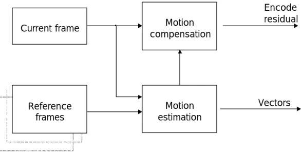
TANDARDS

Motion estimation removes temporal redundancy between successive frames in digital video by creating a model of the current frame, based on available data in one or more reference frames. These reference frames may be earlier or later than the current frame in temporal order. As shown in Figure 2.1, motion estimation creates a model by modifying one or more reference frames to match the current frame as closely as possible according to matching criteria. The current frame is motion-compensated by subtracting the model from the frame to produce a motion- compensated residual frame. This is then coded and transmitted.

Vectors

Current frame Motion

compensation

Motion estimation Reference

frames

Encode residual

Figure 2.1 Estimation and compensation block diagram

(25)

2.2.2 B

LOCKING

M

ATCHING

In the MPEGs and H.263 video standards, motion estimation is carried out on 8 x 8 or 16 x 16 blocks in the current frame. The basic operation of block matching is to divide the image into non-overlapping blocks, and search for the best candidate image block in the reference image frame by calculating and comparing the matching functions between the current block in the current frame and all the candidate blocks within the search area in the reference frame.

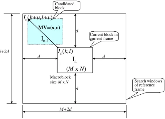
Figure 2.2 illustrates the basic principle of block matching. Block In(k, l) is defined as the pixel intensity at location (k, l ) in the n^th current frame, and block In-1(k+u, l+v) is the pixel intensity at location (k+u, l+v) in the (n-1)^th reference frame.

Suppose the block size is M x N pixels and the maximum displacement of a motion vector is d in both horizontal and vertical directions. A motion vector (u, v) is obtained by finding a matching block within a search window of size (M+2d) x (N+2d) in the reference frame.

(26)

MV=(u,v)

I

_n-1

I

_n

I

_n

(k,l) I

_n

(k+u,l+v)

(M x N)

Current block in current frame

Macroblock

size Mx N Search windows

of reference frame d

d d

d

N+2d

M+2d Candidated block

Figure 2.2 Block-matching diagram

The best-matched block is determined using distance criteria between the blocks in the current frame and the search area blocks in the reference frame. The motion estimation process determines the best dis placement motion vector (MV) by trying to minimize the energy within the search window.

2.2.3 M

OTION

V

ECTORS

The motion of each block is represented by a motion vector, defined as the relative displacement between the current block and the best matched block within the search window in the reference frame (In-1).

Assume that (k, l) is the position of the upper-left corner of a macroblock in the current frame (In) at time (t), as shown in Figure 2.2. If the best matching macroblock in a reference frame is located at (k+u, l+v), the motion vector

(27)

terms, this vector is expressed as (u, v). The vector is a forward motion vector if the reference is an earlier frame (In-1) time (t-1). Conversely, it is a backward motion vector if the reference frame (In+1) is at a later time (t+1).

2.2.4 M

OTION

E

STIMATION

P

ROCESS

The motion estimation process is the search for the best matching macroblock in the reference frame. The best-matched be determined in many ways as criteria functions. One common, computationally simple method is to find block for which the absolute difference between the pixels in the two frames in minimal. The accuracy of motion estimation depends on the matching criteria, and one of the most popular criteria is the SAD(Sum of Absolute Difference). When the value of SAD(u, v) is minimum, (u, v) stands for the motion vector of block in the search area.

2.2.5 M

ATCHING

C

RITERIA

The best-matched block is decided by using a distance criterion between the current blocks in current frame and search area blocks in reference frame. The accuracy of motion estimation depends on the matching criteria applied in the search procedure. The selection of the matching function has a direct impact on the computational complexity and the coding efficiency.

The block match criteria include the sum of absolute difference(SAD), the mean square error(MSE), the mean absolute difference(MAD), and the pixel difference classification(PDC). These matching criteria are defined as below:

2.2.5.1 SAD

SAD seems to be the most popular choice in designing practical image coding systems because of its good performance, relatively simple hardware requirements, and the simplicity of operations required. The SAD is given by

) ,

( ) , ( )

,

; ,

( ₁

1 1

v j l u i k I j l i k I v

u l k

SAD _n _n

N

M + + − + + + +

=

∑

⁻

∑

⁻ ₋ (2-1)

(28)

Where u and v are defined in the search region, –d ≤ u, v ≤ d. In is a sample of the current block, In-1 is a sample of the reference block in the reference frame. The d is maximum search range, the search area is (M+2d) x (N+2d). In(k+i, l+j) denotes the block at location(k, l) in the current frame. In-1(k+i+u, l+j+v) denotes the block at location(k+u, l+v) in the reference frame. When the value of SAD(u,v) is minimum value, MV(u,v) stands for the motion vector of block in the search The motion vector MV(u,v) is given by

MV(u,v) = argmin_(u,v)∈S SAD(u,v) (2-2)

For SAD, we need M x N subtractions, M x N absolute operations and M x N additions to compute one point of m otion vector(MV).

2.2.5.2 MSE

J. R. Jain and A. K. Jain [2-21] propose to apply the mean-squared error (MSE).

The MSE provides a measure of the energy remaining in the difference block. The MSE for an M x N block is defined as

[

¹

]

²

1

0 1

0

) ,

( ) , 1 (

) ,

; ,

( I k i l j I k i u l j v

v MN u l k

MSE n n

N

j M

i

+ + + +

− + +

= −

−

=

−

=

∑

(2-3) The motion vector MV(u,v) is given by

MV(u,v) = argmin(u,v)∈S MSE(u,v) (2-4) However, the MSE criterion is not commonly used in VLSI implementation because it is difficult to realize the square operation in hardware.

2.2.5.3 MAD

Koga et al. propose to use the mean of the absolute frame difference(MAD) [2- 20]. The MAD is given by.

[

⁽ ^, ⁾ ⁽ ^, ⁾

]

) 1 ,

; ,

( ₁

1

0 1

0

v j l u i k I j l i k MN I

v u l k

MAD _n _n

N

j M

i

+ + + +

− + +

= −

−

=

−

=

∑

(2-5)

The motion vector MV(u,v) is given by

(29)

MV(u,v) = argmin(u,v)∈S MAD(u,v) (2-6)

2.2.5.4 MPC

It is well known that the performance of the MAD criterion deteriorates as the search area becomes larger due to the presence of several local minima. Another alternative is the maximum matching pixel count (MPC) criterion. In this approach, each pixel within the matching block is classified as either a matching pixel or a mismatching pixel according to

Otherwise

t j v l i u k I j l i k I v if

u l k

T

ⁿ

+ + −

ⁿ

+ + + + ≤

 

=  ( , )

⁻

( , )

0 ) 1 , : ,

(

¹

(2-7)

Where t is a predetermined threshold. Then the number of matching pixels within the block is given by

) , : , ( )

,

; , (

1

0 1

0

v u l k T v

u l k MPC

N

j M

i

∑

⁻

=

−

=

= (2-8)

The motion vector MV(u,v) is given by

MV(u,v) = argmin_(u,v)∈S MPC(u,v) (2-9) That is, the motion vector MV(u,v) gives the highest number of matching pixels.

The MPC criterion requires a threshold comparator, and a log2(M x N) counters.

(30)

2.3 PERFORMANCE MEASURE PARAMETERS

In order to evaluate the performance of the motion estimation algorithms, the measurement criteria be decided. The most widely used objective measure is peak signal to noise ratio (PSNR). The PSNR is defined as follows:

(2-10)

Where MSE (Means Square Error) is defined as follows:

[

1

]

²

1

0 1

0

) , ( )

, 1 (

) ,

( I k l I k l

l MN k

MSE _n _n

N

j M

i

−

=

−

=

−

=

∑ ∑

(2-11)

Where MN is image size, In(k, l) and In-1(k, l) denotes the original frame and reconstructed frame, respectively. The value 255 is due to the peak value of an 8- bit quantized pixel. This value means the peak intensity value of the video signal.

The PSNR is a used as a method of comparing the quality of video images. For a given image or image sequence, high PSNR indicates relatively high quality.

However, a particular value of PSNR does not necessarily equate to an absolute subjective quality. The PSNR measure is widely used as an approximate objective measure for visual quality and so we will use this measure for quality comparison in this thesis.

2.4 BLOCK-MATCHING ALGORITHMS

For a typical real-time video application with d= 15, f=30, M=352 and N=288 (CIF), full-search(FS) motion estimation requires a computational load of 9.34 billion integer arithmetic operations (with 8- and 16-bit data) per second, as well as a memory bandwidth of 6.22 billion 8-bit accesses per second. Thus, this is an extremely computationally intensive task.

The FS algorithm finds a global optimal motion vector from all the candidate

[ ]

^dB

PSNR MSE 



 



= ₁₀  255 ²

log 10

(31)

real-time visual mobile communication applications. Many fast motion estimation algorithms with reduced computational complexity have been proposed, based on the following approaches: reduction of the number of search points in the search window, reduction of SAD matching (low complexity matching criteria) or pixel decimation, and reduction of search window resolution.

In this section, we investigated and described several famously fast block- matching algorithms, TSS, NTSS, FSS, and BBGDS algorithm.

2.4.1 F

ULL

S

EARCH

(FS)

The conceptually simplest method to find the motion vector, but the most compute-intensive search method, known as the full search (FS) algorithm. In order to find the best matching block in the reference frame, motion estimation is carry out a comparison of the current block with every possible block of the reference frame. In fixed block size full search block-matching, the motion of a block of M x N pixels centered at point (k, l) within a frame interval is estimated. If the maximum search range is d, the number of checking points required is (2d+1)² for the motion vector.

The high computational requirements of FS make it unacceptable for many real time image sequence-coding applications, but the FS provides simplicity and ease of hardware implementation.

2.4.2 T

HREE

S

TEP

S

EARCH

(TSS)

The TSS algorithm is proposed by Koga [2-1]. This algorithm is based on a coarse-to-fine approach with logarithmic decreasing in step size. In the first searching step, the TSS compares the nine search points with a step size equal to or slightly larger than half of the maximum search range, and the TSS selects the minimum SAD. This minimum point becomes the center of the next step. In the second searching step, the step size is halved and eight new candidates located again on the square borders are calculated. For each searching step, the step size

(32)

The above procedure is repeated until the step size is smaller than one and the final motion vector is thus found. Each step has to be performed sequentially.

For searches with 3 steps or d= 7, the number of checking points required is 25.

For larger search windows, the TSS can be easily extended to an n-step search using the same search strategy with the number of checking points required expressed by Equation (2-12).

NCP = [1+8*log2(d +1)] ( 2-12) Here below the advantages and disadvantages of this algorithm are listed by analyzing not only the quality/computational complexity trade-off but also the complexity in terms of generating the candidate motion vectors and the memory bandwidth that must be provided to fetch the searching window pixels from an external memory.

This algorithm has advantages: Low complexity in terms of candidate to evaluate (logarithmic increase with d) and good regularity in terms of motion vector generation. The disadvantages are complex factor slightly increasing with search area, high data bandwidth for all the search area memory data must be accessed, and performs reasonably well on general sequences but has some drawbacks for sequences with limited motion or step increases linearly with d that increases the chance to fall in local minimum.

This algorithm uses a uniformly allocated search pattern in its first step, which is not efficient to catch small motions or center-biased motions [2-12].

2.4.3 B

LOCK

B

ASED

G

RADIENT

D

ESCENT

S

EARCH

(BBGDS)

The block-based gradient descent search (BBGDS) algorithm has been proposed by literature [2-4]. Based on the observation that global minimum distribution is centralized in real video sequence, this algorithm uses a very center- biased search pattern of nine checking points in each step with a step size of one.

It does not restrict the number of searching steps but it stops when the minimum

(33)

checking point of the current step is the central one or it reaches the search window boundary.

There are also overlapped checking points between adjacent steps. This algorithm performs better for searching small motions and offers the big advantage of using a half-way stop mechanism. In fact, it can save lot of processing power in simple sequences. The average number of checking points is given by equation 2- 13, where the a factor is the mean overlap factor between two steps which is bounded by the value 3 (horizontal or vertical overlap) and 5 (diagonal overlap):

NCP = [9+a*Step] ( 3 = a = 5) (2-13) This algorithm has advantages: very low complexity in terms of candidate to evaluate, good regularity in terms of motion vector generation, and only portion of search area memory can be accessed (memory bandwidth saving)

The disadvantages only possible for steady-like scene and unable to catch high motion vector, unless very large number of steps are used since it can be easily trapped in local minimum when large motion occurs.

The BBGDS searches for motion vectors along the direction where the minimum SAD is expected to lie. The BBGDS algorithm performs better in searching center- biased or small motions, the computational complexity is significantly less than that of the TSS and the NTSS [2-4].

2.4.4 N

EW

T

HREE

S

TEP

S

EARCH

(NTSS)

The new three-step search algorithm (NTSS) is proposed by [2-12], [2-19]. It is a modified version of the three-step search algorithm to improve the quality for small motion video sequences occurring mostly in video conferencing applications.

For those video sequences, the motion vector distributions are highly center biased. Therefore, eight additional checking points, centered on the origin are searched in the first step of NTSS. If the minimum is indeed center biased, the

(34)

is not located in the eight additional points, the algorithm behaves exactly as the three-step search.

The number of checking points for the worst case is given by equation 2-14.

NCP = [9+8*log2 (d +1)] (2-14)

This algorithm has advantages: low complexity in terms of candidate to evaluate, obtain high quality at very low processing power for center biased motion scene.

The disadvantages are candidate vector generation slightly more sophisticated than TSS algorithm, complexity factor increasing with search area, risk of local minima if motion not centered around (0, 0), and high data bandwidth.

2.4.5 F

OUR

S

TEP

S

EARCH

(FSS)

The four-step search algorithm (FSS) is proposed by [2-2]. The algorithm is also exploits the center-biased characteristics of the real world video sequences by using a smaller initial step size compared to TSS. The initial step size is a quarter of the maximum motion displacement d. Due to the smaller initial step size, the FSS algorithm needs four searching steps to reach the boundary of a search window with d =7. Similarly to the small motion case in the NTSS algorithm, the FSS algorithm also uses a halfway stop technique in its second and third step search.

Moreover if the minimum searching point is found to be the central one, the step size is halved and the process jumps to the fourth step. In the general case the algorithm can be extended as follows: if the step size of the fourth step is larger than one, another four-step search is performed with the first step equal to the last step of the previous search. The number of check-points required for the worst case is

NCP = [9+18*log2(d +1)/4]] (2-15)

(35)

The advantages are very low complexity in terms of the candidate to evaluate, faster convergence than BBGDS if the motion vector is far from (0, 0), and only portion of search area memory can be accessed for memory bandwidth saving.

This algorithm has disadvantages; more complex than BBGDS if motion is close to (0, 0), risk of local minimum if motion is far away from (0, 0).

2.5 MOTION ESTIMATION ALGORITHMS COMPLEXITY

Optimization of motion estimation algorithm has been widely studied because of its fundamental impact on compression efficiency, and motion estimation’s high requirements for both processing power and data bandwidth. Each time that a new candidate motion vector is generated, its fitness must be evaluated by matching the two macroblocks. This process is repeated until a final motion vector with minimal cost is found. The complexity cost of performing motion estimation for a macroblock is given by the following equation:

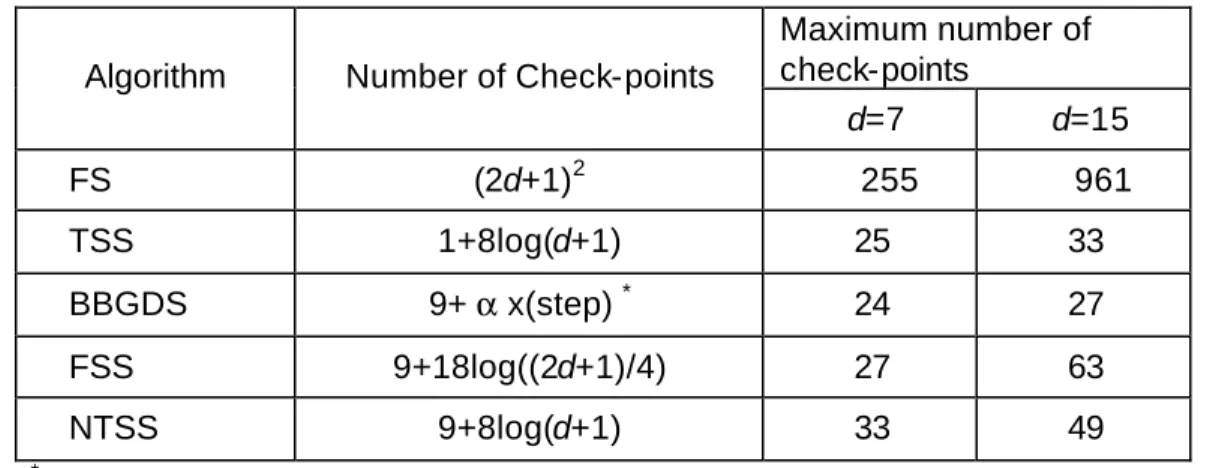
Complexity(MB) = [ (MxN) x Cpixel ] x NCP + Ccontrol (2-16) This equation shows that the complexity is proportional to the number of check- points(NCP), the size of pixels used to perform the match (M x N), and the complexity to evaluate one pixel match (Cpixel), CControl is the additional control complexity of motion vector generation. The numbers of check-points (NCP) for each algorithm are summarized in Table 2.1. Existing fast motion estimation algorithms can be roughly divided into three approaches according to the complexity equation:

1) Fast matching obtained by pixel decimation (M, N reduction).

2) Fast search by reduction of motion vector candidates, including many conventional fast search algorithms (NCP reduction).

3) Reduced search window resolution with hierarchical approaches (NCP, M, N reduction).

(36)

We analyzed complexity based on the maximum number of check-points for candidate algorithms. The establishment of rigid metrics for complexity analysis is a difficult task. We investigated check-points as a measure of computational complexity.

As shown in Table 2.1, the check-points are dependent on search area and block size. Even if the check-points are dependent on the characteristics of the images, the BBGDS algorithm has the least number of check-points among the algorithms examined.

The sizes of image and block, search range, and matching criterion have a strong impact on the performance and computational complexity of the motion estimation results. These parameters also have a strong impact on the VLSI cost.

Table 2.1 The computational complexity for algorithms.

Maximum number of check-points

Algorithm Number of Check-points

d=7 d=15

FS (2d+1)² 255 961

TSS 1+8log(d+1) 25 33

BBGDS 9+ α x(step) ^* 24 27

FSS 9+18log((2d+1)/4) 27 63

NTSS 9+8log(d+1) 33 49

( ^*α means overlap factor between two steps which is bounded by the value 3(horizontal or vertical overlap) and 5 (diagonal overlap), 3< α < 5. The step means the number of search step. Here we assume, the step is 3, 6 at d=7, d=15 respectively)

(37)

2.6 PROPOSED ALGORITHM

2.6.1 B

ASIC

C

ONCEPT

The contents and characteristics of images vary in the image sequences.

Adaptive s election of the algorithm of motion estimation according to image characteristics results in better performance and efficiency.

Before we described the two searching methods that the one algorithm likely BBGDS is more center-biased and converges more rapidly when the best match is close to the center of a search. On the other hand, the other algorithm performs better when the best match is located far from the center of the search. The assumption is that if the majority of the motion decisions involve small motions, it is likely that the current block also has a small motion, in which case a more center- biased algorithm will be the better choice. In addition, the same argument holds when the majority of the motion is large.

The new algorithm selects the best motion estimation algorithm according to motion type. To choose between the two different kinds of searching method, motion is classified as large or small; the motion type is determined by checking the motion vector and SAD.

(38)

2.6.2 A

LGORITHM

We firstly investigated two kinds of algorithms, TSS algorithm and BBDS algorithm. For the TSS algorithm, the best-case number of search points depends only on the search window size, and remains the same, irrespective of the distance from the center for a given search window size.

The number of search points for the TSS algorithm changes only when the searching range changes. From in the Table 2.1, for a 16 x 16 search window, the TSS requires 25 search point comparisons, while for a 32 x 32 search window, the TSS requires 33 search point comparisons for any point.

While the best-case number of search points for BBGDS always increases with distance from the center, this is also dependent on the search window and search step size. This algorithm requires the largest number of search points at the corners of the search square. The algorithm requires a minimum of 9 and a maximum of 19 search points for a step size of 3.

We proposed two kinds of search patterns, center-biased search and noncenter-biased search.

For center-biased search, we modified based on the BBGDS algorithm. For BBGDS, the search proc edure stops when it reaches the search window boundary.

The number of search points is dependent on search window size. But, we modified the algorithm such that the search stops when the minimum checking point of the current step is the central one or after only three steps in the all search windows size.

For non-center-biased search, we also modified based on the TSS algorithm.

The modified uses a uniformly allocated search point pattern in its first step. Then, the first step size changes half of the maximum motion displacement (d/2) to 8.

The maximum number of search points is 25 and this is independent of search window size. In the thesis, we fixed the search pattern in the first step, the search pattern is start with fixed initial step size is 4, and stops after only three steps in the

(39)

all search windows size. In this case, the performance is similar to that of the TSS algorithm. We simplified and optimized the search pattern.

2.6.3 M

ETHOD OF

M

OTION

S

ELECTION

We developed an algorithm for adaptive selection of the appropriate block- matching algorithm for varying motion content. The selection process is as follows:

Step 1. Calculate the SAD0 at the original point.

Step 2. Compare the SAD with a threshold (TH).

If the SAD < TH, select the center-biased search, classify the motion characteristics as small motion and proceed to Step 3. Otherwise, select the noncenter-biased search, classify the motion characteristics as large motion and proceed to Step 3.

Step 3. Search the motion vector (MV), using the selected algorithm.

The different searching methods are chosen on a block-by-block basis. Small motion was defined as that in which the motion vectors are within a 3 x 3 window, and large motion was defined as that in which the vectors are outside a 3 x 3 window. These definitions are used throughout this thesis to distinguish between small and large motion vectors.

Our algorithm combines the ability of the noncenter-biased algorithm to cover good searches for large motion sequences with the center-biased nature and search speed of the center-biased algorithm.

(40)

2.7 PROPOSED ARCHITECTURE

Here, we describe the proposed hardware architecture for implementing our proposed algorithm. This hardware architecture employs two kinds of block- matching search patterns, selected on the basis of the block address, pixel address, and search controls.

2.7.1 A

LGORITHM

M

APPING

The proposed algorithm calculates nine candidate blocks in each of three search steps. The proposed two searching patterns consist of the same three nested loops: Loop 1 is for each of the search steps, Loop 2 is for each of the nine candidate positions of motion vectors, and Loop 3 calculates the absolute pixel differences.

The search pattern and data flow for the two searching patterns are very similar.

The candidate search blocks are data-dependent, which means that the result of the current step determines the search blocks to be evaluated in the next step.

Therefore, each step has to be performed sequentially.

We can parallel Loop 2 by using nine PEs with a single PE calculating the SAD of one of the nine search positions, sequentially execute the operations in each step of Loop 1, and calculate the pixels in Loop 3.

The architecture can be changed by altering the values of counters in Loops 1 and 3 for a different search range and block size, which does not affect the hardware architecture. We implemented two searching methods by selecting the block address, pixel address, and search controls.

(41)

2.7.2 B

ASIC

S

TRUCTURE

The general architecture of motion estimation consists of a processing element, memory (search area and current block), a memory controller, and an MV detector module.

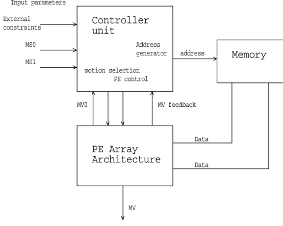
Our proposed architecture is shown in Figure 2.3; it consists of three main parts:

a control unit, a PE array unit, and memory. The control unit has a number of sub- modules: parameter control, memory-addressing control and generator, PE control unit, and motion selection. The PE array consists of nine PEs, which can operates in parallel, and the memory consists of nine banks.

PE Array Architecture

address

MV Input parameters

MV0

PE control Address generator

Controller unit

Data

Data External

constraints MS0

Memory

MS1

MV feedback motion selection

Figure 2.3 Block diagram of flexible motion estimation

(42)

The control unit controls address generation, PEs, input parameters, and motion selection. The address generator calculates the start and the next address of data in memory, and interfaces with external memory. This consists of an adder, register, and multiplier. If the address generator is programmable, a different algorithm can be implemented in the same architecture, and the hardware architecture is thus highly flexible. In motion selection, to select the better algorithm, the SAD is compared with the threshold (TH), and then the result is input into the address generator unit. The PE controller controls PEs for power management and can be enabled or disabled on operating PE units.

The input parameters have external constraints, MS0 and MS1. The external constraints can be input as system requirements and constraints for power and performance. MS0 and MS1 can be used to select the architecture and algorithm mode, for example, block-matching algorithms that use sub-sampling of pixels with a block size of 8 x 8 or 16 x 16. These parameters can be used to control the algorithm and optimize the architecture.

2.7.3 P

ROCESSOR

E

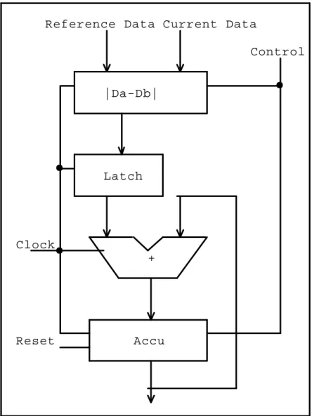
LEMENT

A

RRAY

Figure 2.4 shows a single PE unit. The PE unit performs the subtraction, absolute value, and partial sum addition. A PE has reference data input ports, current data input ports, clock, reset, and control signals. Each PE unit has a clock with the appropriate data from memory. This PE unit calculates the sum of all absolute differences until an external signal resets the accumulator of the SAD summation.

(43)

|Da-Db|

Control

Clock

Latch

Reset Accu

Reference Data Current Data

+

Figure 2.4 SAD PE element

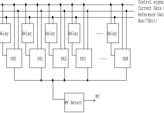
Motion estimation can be parallelized at the PE level, with each PE unit calculating the PE of a single motion vector candidate. The PE array can be one- or two-dimensional. We selected a 9 x 1 one-dimensional PE array (Figure 2.5) for mapping our algorithm to the hardware architecture. The TSS and the BBDS algorithms calculate nine candidate check-points in each search step. We can

(44)

parallel calculation of the SAD of one of the nine search positions, sequentially execute the operations in each step, and calculate pixels.

The PE control signals can be from a programmable delay unit and can enable or disable PE units. An MV detection unit is used to find the minimum SAD and can determine when to stop a search procedure.

Current Data Bus(8bit) Reference Data

Bus(72bit)

PE8 delay

PE2

Control signals

delay

---- PE3

delay ----

PE1 delay

PE0

delay

MV detect

MV

Figure 2.5 PE array with nine PEs

(45)

2.7.4 A

DDRESS

G

ENERATION

U

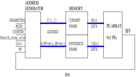
NIT

The address generation unit is an important part of the hardware design for implementing multi-motion estim ation algorithms. This unit consists of a multiplier, adders, counters, and registers. The unit address memory is used to compute the SAD and motion vector, and the address generator can provide the base address of the next step when each PE is calculated at the nine check-points. Thus, the correct address can be picked out immediately after the minimum SAD is decided.

The unit controls the search pattern of the algorithms and assigns search points by selecting the block address and pixel address within the block. By changing the design of this unit, different search algorithms can be implemented in this architecture. Use of a programmable device would provide future flexibility.

However, we did not use a programmable device, but utilized parameters for algorithm s election to implement hardware simply without a great deal of overhead.

Search_step_size

Functionality MS0/MS1

MV

register

0 0

1 1 Parameters

1 0 ADD

8 8

address

0 1 +

No pel sub-sampling

block size 16x16 MUX

(0,1,2,4,8)

MS0/MS1

counter

Algorithm mode

block size 8x8

Memory address

2:1 pel sub-sampling

(a)

(46)

REFERENCE FRAME

8bit DATA C(i,j)

PARAMETERS MODE

Init

9x1 PEs

ADDRESS MV

CURRENT FRAME MEMORY

MV

72bit DATA ADDRESS

GENERATOR

Search_step_size

PE ARRAY COUNTER

R(MV+m+i,MV+m+j)

(b)

Figure 2.6 Address generation unit

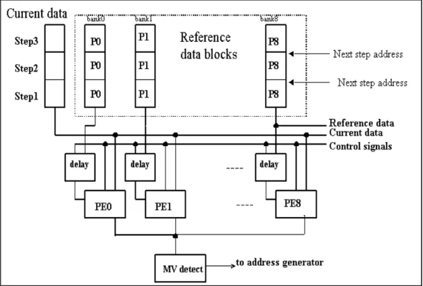
2.7.5 D

ATA FLOW

Figure 2.7 shows the basic PE array structure and its input data flow. The current frame data are broadcast sequentially to all nine PEs simultaneously from a single data bus and are identical for all nine PEs. The reference data are different for each PE, and therefore the reference data are broadcast from each memory bank to a single PE from a separate data bus.

The proposed algorithm requires 256 cycles at each search step to calculate the SAD. Each macroblock can be processed in 768 (256 x 3) cycles. The memory bandwidth is 7680 (256 x 3 x 10). This structure requires nine memory banks without memory partitioning schemes or scheduling. It is possible to reduce the memory bank requirements by using memory partitioning, data reuse, and scheduling, but this would mean that we would no longer be able to complete the search within 768 cycles. This structure is also expandable as different search range, block size, and search step.

(47)

It is necessary to find reasonable tradeoffs among the array size, area, required cycle, bandwidth, and power consumption. This was simplified for implementation using VHDL.

Figure 2.7 PE Array Block Diagram.

(48)

2.8 IMPLEMENTATION RESULTS

We evaluated various algorithms implemented in C language. We compared the FS, TSS, BBGDS, and our proposed algorithms in terms of average peak signal to noise ratio (PSNR) for quality and CPU times (seconds) for computational complexity. The algorithms were run ten times on a 200MHz UltraSparc processor with 128MB of memory.

2.8.1 Q

UALITY

C

OMPARISONS

The PSNR was used to evaluate the quality of a reconstructed image sequence quantitatively. The PSNR is given by equation 2-10 and equation 2-11. Simulations were performed using various test image sequences, i.e., “HALL” (352 x 288/176 x 144 pixels), “Football” (352 x 240 pixels), “Tennis” (176 x 144 pixels), and “Mobile”

(352 x 240 pixels). Each sequence included 80 frames. The search range was –15 to 16 pixels, and the block size was fixed at 16 x 16 pixels for both the horizontal and vertical directions.

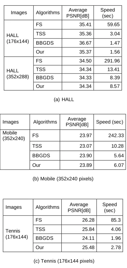
Our proposed algorithm was simulated with the TSS, BBGDS, and FS algorithms, and the PSNR performances and speed of the different algorithms were compared. Table 2.2 shows the results of the PSNR comparison for the four algorithms for the test image sequences. These results indicate that the PSNR and average search times of our proposed algorithm were always very close to those of the best algorithm. Our proposed algorithm did not always perform better than TSS or BBGDS, but its performance was always better than the worst of the two and comparable to the better of the two. Our algorithm was faster than the TSS, but slightly slower than BBGDS. Our algorithm can be used across different types of motion and formats to provide good tradeoffs in terms of quality and speed. In addition, our algorithm can be extended to replace BBGDS with other center- biased block-matching algorithms, and the TSS with other search strategy block- matching algorithms.

(49)

Table 2.2 Average PSNR and Speed Comparisons for Four Algorithms.

Images Algorithms Average PSNR[dB]

Speed (sec)

FS 35.41 59.65

TSS 35.36 3.04

BBGDS 36.67 1.47

HALL (176x144)

Our 35.37 1.56

FS 34.50 291.96

TSS 34.34 13.41

BBGDS 34.33 8.39

HALL (352x288)

Our 34.34 8.57

(a) HALL

Images Algorithms Average

PSNR[dB] Speed (sec) Mobile

(352x240) FS 23.97 242.33

TSS 23.07 10.28

BBGDS 23.90 5.64

Our 23.89 6.07

(b) Mobile (352x240 pixels)

Speed (sec)

FS 26.28 85.3

TSS 25.84 4.06

BBGDS 24.11 1.96

Tennis (176x144)

Our 25.48 2.78

(50)

Speed (sec) Football

(352x240) FS 26.49 313.71

TSS 26.01 13.96

BBGDS 26.13 6.59

Our 26.16 7.26

(d) Football (352x240 pixels)

17 22 27 32 37

1 6 11 16 21 26 31 36 41 46 51 56 61 66 71 76

Frame Number PSNR[dB]

TSS BBDS

OUR FS

(a) Tennis (176x144)

21 23 25 27 29 31

1 6 11 16 21 26 31 36 41 46 51 56 61 66 71 76

Frame Number

PSNR[dB] TSS BBDS

OUR FS

(b) Football (352x240)

(51)

22 23 24 25

1 5 9 13 17 21 25 29

Frame number

PSNR[dB] TSS BBDS

OUR FS

(c) Mobile (352x240)

Figure 2.8 PSNR Comparisons.

(52)

2.8.2 P

ERFORMANCE

A

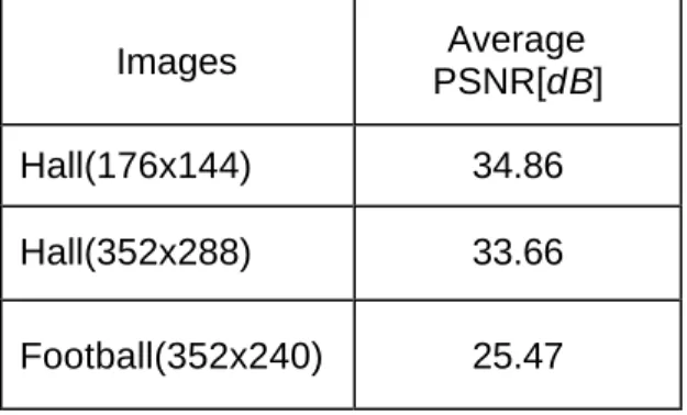
NALYSIS

Table 2.3 lists the average PSNR for our proposed architecture. The block size was 16x16, the search range was -15/+16.

Table 2.3 Results of Performance Analysis (Search range -15/+16; block size 16x16)

Images Average

PSNR[dB]

Hall(176x144) 34.86 Hall(352x288) 33.66 Football(352x240) 25.47

(53)

2.8.3 VLSI Implementation

The proposed architecture was designed using VHDL Synopsys design tools and 0.35µm Hitachi CMOS technology. The implementation results are summarized in Table 2.4. The clock rate was constrained to 20ns.

Table 2.4 Features of the VLSI Architecture Technology 0.35µm Hitachi CMOS

PE Array 0.5486[mm²] Controller 0.05621[mm²] Chip

size

0.60481[mm²]

Clock frequency 50Mhz

Our architecture implements two different search methods. Generally, our proposed algorithms require less chip area and lower power consumption than the FS algorithm. The proposed architecture offers both flexibility and less overhead than the other architectures.

Studies on Hardware/Software Codesign Methodology for Video Encoders

Studies on Hardware/Software Codesign Methodology for Video Encoders

ビデオエンコーダを対象とした

ハードウェア/ソフトウェア協調設計方法に関する 研究

March, 2003

Jinku CHOI

崔 鎮 求

Studies on Hardware/Software Codesign Methodology for Video Encoders

ビデオエンコーダを対象とした

ハードウェア/ソフトウェア協調設計方法に関する研究

March, 2003

Department of Electronics, Information & Communication Engineering

Graduate School of Science and Engineering Waseda University

早稲田大学院 理工学研究科 電子・情報通信学専攻

システムVLSI研究

Jinku CHOI

崔 鎮 求

STUDIES ON HARDWARE/SOFTWARE CODESIGN METHODOLOGY FOR VIDEO

ENCODERS

By Jinku CHOI

Department of Electronics, Information & Communication Engineering

Graduate School of Science and Engineering Waseda University

Under the Supervision of Prof. Dr. Tatsuo OHTSUKI

March, 2003

2002

All Rights Reserved

TABLE OF CONTENTS

Table of Contents

List of Tables

List of Figures

Chapter 1 Introduction

Chapter 2 Selection Based Algorithm and Architecture for Motion Estimation

Chapter 3 Hardware/Software Implementations of Video Encoders

Chapter 4 Hardware/Software Codesign Methodology for Video

Encoders

Chapter 5 Conclusions

References

Publications List

LIST OF TABLES

LIST OF FIGURES

CHAPTER 1

INTRODUCTION

CHAPTER 1 INTRODUCTION

CHAPTER 2

SELECTION BASED ALGORITHM AND

ARCHITECTURE FOR MOTION ESTIMATION

CHAPTER 2 SELECTION BASED ALGORITHM AND ARCHITECTURE FOR MOTION ESTIMATION

2.2.1 M

-C

C

S

2.2.2 B

M

I

I

I

(k,l) I

(k+u,l+v)

(M x N)

2.2.3 M

V

2.2.4 M

E

P

2.2.5 M

C

2.2.5.1 SAD

∑

∑

2.2.5.2 MSE

[

]

∑

∑

2.2.5.3 MAD

[

]

∑

∑

2.2.5.4 MPC

ハードウェア/ソフトウェア協調設計方法に関する研究

崔鎮求

早稲田大学院理工学研究科電子・情報通信学専攻

崔鎮求