富 山 大 学 紀 要. 富 大 経 済 論 集 第62巻第 1 号抜刷(2016年7月)
富山大学経済学部
Guoqing ZHAO, Tao WEN, and Jun MA
Impact of Financial Development and Foreign Direct Investment on Investment Allocation Efficiency in China
: An Evidence Based the Industrial Panel Data
Impact of Financial Development and Foreign Direct Investment on Investment Allocation Efficiency in China
: An Evidence Based the Industrial Panel Data
Guoqing ZHAO, Tao WEN, and Jun MA*
Abstract: Using China’s provincial panel data set containing 17 industries from 2006 to 2012, we assess the effect of financial development and foreign direct investment (FDI) on the allocation of China’s industrial investment, based on two investment allocation efficiency indicators, the industrial sales elasticity of total fixed assets and the industrial value added elasticity of total fixed assets, respectively. When using the sales elasticity of total fixed assets to indicate investment allocation efficieng, we find that FDI and stock market activities had negative effects while investment allocation efficiency was spurred by domestic bank loan whose impact was largely reduced by FDI, and loan to the private sector had a mild influence on investment allocation efficiency. Contradictory results are obtained by using industrial value added elasticity of total fixed assets as the indicator of the investment allocation efficiency, which could be attributed to the fact that China's FDI was below the minimum threshold value to fully promote the optimization of domestic bank loan but reached that for loans to the private sector. Furthermore, stock market has a positive effect on investment allocation efficiency and barely any crowding out effect on FDI.
Therefore, policy-makers should carefully consider the economic condition, the development plan and location when choosing the optimal investment scheme, and gradually switch the sales-driven investment strategy to that aiming at increasing industrial value-added.
Key Word:Foreign direct investment (FDI); Financial development;
Investment Allocation Efficiency
JEL Classification: C31, F21, G11
* Guoqing Zhao([email protected]) and Tao Wen, School of Economics, Renmin University of China, Beijing, 100872,China. Jun Ma([email protected]), Department of Business Administration Faculty of Economics, University of Toyama, Japan, 930-8555.
1. Introduction
China experienced amazing high growth rate of GDP in the past decade, most of which was contributed to the increased investment in the fixed asset. For example, in 2013, the proportion of total investment in fixed assets in GDP was 78.46 %, and the total fixed assets investment grew by 19.1%. In 2014, the final consumption expenditure accounted for only 37.3% of the GDP in China, while this ratio was 68.5% in the USA and was above 75% in other developed countries such as Britain, Germany, and Japan. In other words, there exists an issue of excessively high investment rate in China's GDP structure. The economy needs to maintain a certain growth rate of investment, which is the driving force of economic development, but over-investment and excessive investment growth may induce pivotal problems related to credit expansion, land finance, excess capacity and so on, and lead to the imbalance of economic structure and atrophy of the residents' consumption.
Investment-led GDP has become a practical circumstance in China, which is difficult to be reversed in the short term. Hence, the government should improve the efficiency of investment when restructuring the economy gradually, because high investment allocation efficiency could effectively promote the development of economy. When considering the investment allocation efficiency, a prevailing assumption is that "the best form of investment is to increase investment in growing industries and reduce investment in declining industries". That is, if investment flows to the industries with high expected return and withdraws from the industries with low expected return, the investment is efficient. Based on this assumption, many scholars study the domestic or transnational economic investment allocation efficiency, and analyze the related factors
that influence the investment allocation efficiency.
When it comes to investment allocation efficiency, we should clarify the sources of investment first. In general, there are five main capital sources for fixed assets investment, i.e., stafe budget, domestic loans, foreign investment utilization, self-raising funds and other investment. From the statistical yearbook, we can find that domestic loans compose a relatively large part in the industrial investment. In 2012, China's non-financial corporate loans increased by 5.66 trillion yuan, while the annual industrial investment was 15.5 trillion yuan, and the bank loan accounted for 36.5
% of the industrial investment. On the other hand, the amount of foreign investment utilization was 111.7 billion dollars, accounting for about 4.7%
of the industrial investment after conversion. As shown in the statistics, bank credit and foreign investment are the two main sources of funds for the investment in industry in China. In addition, compared with self- raising funds, bank credit and foreign investment have great advantages in the sense that they have a clear demand of investment return, which would bring pressure on enterprises and promote the enterprises to improve operation.
One of the most curtail functions of the financial system is to allocate capital efficiently, i.e., to increase investment in the regions or industries with high returns and to reduce investment in area or industries with poor prospects. Financial development contributes to economic growth through a considerable amount of channels such as helping a country take better advantage of its investment opportunities (Wurgler, 2000). The difference in development of financial sector is able to explain a substantial proportion (although not all) of the cross-country variation in the quality of capital allocation. Calderon and Liu (2003) find that financial development
generally leads to economic growth and financial deepening propels economic growth through both a more rapid capital accumulation and productivity growth, with the latter channel being the strongest. However, Rioja and et al. (2004) find that financial development has an uncertain effect on growth in countries with very low levels of financial development and a large, positive effect on growth in countries with intermediate levels of financial development and a positive, but smaller effect in countries with high levels of financial development, respectively. Christopoulos et al. (2004) investigate the long-run relationship between financial depth and economic growth, they claim that financial depth is an important factor in promoting economic growth, but economic growth does not necessarily promote financial depth. Ndikumana (2005) finds that financial intermediation affects domestic investment notably by alleviating financing constraints, allowing firms to increase investment in response to increased demand for output. Galindo et al. (2007) find that liberalization increases the efficiency with which investment funds are allocated. Islam et al. (2006) examine the impact of financial market development on the extent to which firms rely on internal capital for making investments and find evidence of a negative relationship between financial market development and the importance of internal capital. Pang et al. (2009) explore the channel of capital allocation through which finance promotes economic growth and find that countries with developed financial markets invest more in growing industries, and pull out more funds of declining ones. Morck, Yavuz and Yeung (2011) observe less efficient capital allocation in countries whose banking systems are more thoroughly controlled by tycoons or big families. They find that countries with banking system controlled by tycoon or family have slower economic productivity growth, greater financial instability, and higher
degree of income inequality. Taboada (2011) studies the influence of the change in ownership structure of banks on the capital allocation efficiency, and shows that the decline in government ownership of banks affects capital allocation efficiency differently, depending on whether foreigners or large domestic holders who take over the stakes. In particular, the increase in domestic holder presence in the banking sector hampers capital allocation efficiency while the increased foreign presence in the banking sector leads to improvements in capital allocation.
Another factor which largely affects the allocation of capital is foreign direct investment. Capital of the developed countries usually seeks investment opportunities in other country according to the difference of resources endowment. This investment behavior changes the pattern of capital allocation of the invested country, leading to the increase of capital in the most efficient sectors. Despite numerous theories on this linkage, there is little empirical evidence on whether and how FDI improves the allocation of capital. Harrison et al. (2003) find that foreign enterprises have a spillover effect on domestic enterprises by attracting more bank loans due to their higher profitability and capital mobility. In developing countries, domestic enterprises face a harder credit constraint then the foreign enterprises, which may be released by FDI. However, there are a substantial number of studies suspect whether such spillovers do take place (Wang and Tu, 2007; Chen and Sheng, 2008). Wang (2006) shows that FDI has a technology spillover effect which can be enhanced by the improvements in the financial market efficiency such as lower financial costs and higher capability of labor. Aurangzeb and Stengos (2014) examine the relationship between FDI and economic growth with a smooth coefficient semi-parametric approach. Their results show that countries
with higher levels of FDI inflows have higher productivity, because FDI is not only an important direct determinant of growth, but also a tool helping improve factor productivity in the exports sector.
Financial development and FDI jointly affect the investment allocation efficiency. In other words, the mechanism of the interaction between financial development and FDI plays an important role in improving the efficiency of investment allocation. Yang and Lai (2006) propose a different view by showing that in China, the low efficiency of financial market obstructs domestic enterprises’ acquirement of foreign technology, although FDI has positive effects on accumulation of capital. Sun (2008) finds that financial development can contribute to the domestic capital accumulation and economic growth, encourage more FDI, provide better services to foreign enterprises, and transform the potential FDI spillover effect to real productivity. Lee and Chang (2009) claim that financial development indicators have a larger effect on economic growth than FDI, but in the long-run, FDI coupling with financial development contribute to global economic growth. Pang and Wu (2009) conclude that countries with developed financial market invest more in growing industries and withdraw funds from the industries with lower return, using international industrial data. Alfaro et al. (2010) find that development of the financial market benefits from FDI by economic growth promoted by the increase in FDI.
The essential of the above literature is the indicator of investment allocation efficiency proposed by Wurgler (2000). This investment allocation efficiency indicator is obtained by regressing the investment growth rate of fixed assets and that of the industrial value-added, meaning that one unit of change in the growth rate of the industrial value-added leads to changes in the certain times of the investment growth rate of fixed assets. If the
ratio is positive, the investment will increase as the industrial value-added grows, in which case the investment is efficient; otherwise, the investment is inefficient. The commonly accepted method describes the relationship of capital return rate and investment allocation. Li et al. (2010) follow the original method and conclude that the average investment allocation efficiency indicator of China's various regions is 0.204, and the national overall efficiency indicator is only 0.126, which is far below the number (0.429) of average investment allocation efficiency of 65 countries calculated by Wurgler (2000). The question is: the large investment growth obviously could not be fully explained by the growth of the industrial value-added.
The growth rate of China's fixed asset investment is between 11% - 20% in long-term, but the growth rate of China's industrial added value is always less than 7%, which means the growth rate of fixed asset investment is higher than industrial added value. Hence, Wurgler (2000) ’s investment allocation efficiency indicator does not match the current situation in China, and there should exist a more important factor affecting the fixed assets investment. The characteristic of investment is that capital flows to the industries or regions with high return, and the main representation of the return is the increase of sales volume and profit. Therefore, after the comparison, we consider it is suitable to calculate the investment allocation efficiency with industrial added value and industry sales. This paper contributes to the literature by setting two investment allocation efficiency indicators: sales elasticity of total fixed assets and industrial value added elasticity of total fixed assets. Then, we pay a closer examination on the relationships between financial development, FDI, and investment allocation efficiency in China. We aim at proposing a more proper assessment of the investment allocation efficiency and its determinants
based on China's economy, and providing more constructive suggestions on economic policies.
The paper proceeds as follows. Section 2 discusses data and the measurement of some variables. Section 3 presents empirical analysis.
In Section 4, we test the effect of financial structure on allocation of investment. Finally, Section 5 concludes the paper.
2. Data and Measurement
2.1 Manufacturing industry statistic
The empirical investigation is based on manufacturing industry level panel data for 30 provinces of the Chinese mainland. The sources of the basic manufacturing industry statistics come from China Industry Economy Statistical Yearbook (2006-2012), which provides balance sheet information on 27 manufacturing industries. This paper needs balanced panel, so we require at least three consecutive years of observation on each industry. These criteria leave observation only available for 17 industries. Some provincial characteristics variables, including FDI measurement, information comes from China Statistical Yearbook (2007-2012). The proxies for financial development come from Almanac of China’s Finance and Banking (2007-2012).
Table 1 is the statistical description of industrial sales growth and growth in the industrial added value of 17 manufacturing industries in 30 provincial areas of China Mainland. As shown in the table, both rates are lower in the relatively developed area such as Beijing, Shanghai, and Zhejiang, mainly due to the fact that their level of economic development was relatively high and the infrastructure construction was very complete at the beginning of this period. In particular, these areas had more rational second industry structure, stronger residents' consumption capacity,
smaller price elasticity of demand and income elasticity of demand, and more stable growth in the industry sales and industrial added value.
Also, the tertiary industry had become the main economic composition in these areas; the second industry had lost its dominance; the demand for manufacturing product were reduced.
Table 1. Grouth rate of industrial sales and added value in provincial areas sales growth and investment growth
Province Industry sales growth Industrial value added growth Mean. Std. Dev. Obs. Mean Std. Dev. Obs.
Beijing 0.132 0.161 102 0.106 0.230 102
Tianjin 0.239 0.258 102 0.190 0.313 102
Hebei 0.244 0.117 102 0.207 0.238 102
Shanxi 0.216 0.233 102 0.136 0.228 102
Inner Mongolia 0.383 0.266 102 0.239 0.323 102
Liaoning 0.284 0.162 102 0.174 0.241 102
Jilin 0.355 0.245 102 0.187 0.499 102
Heilongjiang 0.202 0.177 102 0.145 0.519 102
Shanghai 0.129 0.156 102 0.086 0.116 102
Jiangsu 0.232 0.120 102 0.188 0.188 102
Zhejiang 0.174 0.131 102 0.139 0.178 102
Anhui 0.358 0.179 102 0.311 0.527 102
Fujian 0.257 0.146 102 0.197 0.329 102
Jiangxi 0.363 0.184 102 0.267 0.367 102
Shandong 0.229 0.105 102 0.172 0.189 102
Henan 0.323 0.173 102 0.258 0.296 102
Hubei 0.320 0.149 102 0.235 0.345 102
Hunan 0.350 0.153 102 0.245 0.270 102
Guangdong 0.205 0.115 102 0.128 0.215 102
Guangxi 0.378 0.296 102 0.273 0.646 102
Hainan 1.266 4.961 102 1.093 3.470 102
Chongqing 0.301 0.177 102 0.186 0.250 102
Sichuan 0.329 0.172 102 0.276 0.444 102
Guizhou 0.209 0.208 102 0.184 0.473 102
Yunnan 0.249 0.243 102 0.215 0.537 102
Shaanxi 0.285 0.163 102 0.308 0.815 102
Gansu 0.228 0.222 102 0.126 0.610 102
Qinghai 0.549 1.514 102 0.606 5.080 102
Ningxia 0.306 0.583 102 0.272 0.494 102
Xinjiang 0.274 0.277 102 0.214 0.393 102
2.2 Measuring the efficiency in the allocation of investment
Following the approach of Wurgler(2000), in this paper we use growth in total fixed assets to measure growth in investment, and measure the efficiency of capital allocation with two elasticity, industrial sales elasticity of total fixed assets and industrial value added1 elasticity of total fixed assets, both of which could be used as the form of investment elasticity that “assumes that optimal investment implies increasing investment in industries that are growing and decreasing investment in industries that are declining”. The difference is that we estimate the elasticity of investment for each year in each province in China, comparing to the elasticity for each country in Wurgler (2000) or the elasticity of investment for each industry in each countries in Pang and Wu (2009).
We estimate the following simple specification of industrial sales elasticity of total fixed assets for each province in each year:
ipt ipt pt
pt
ipt
GSALES
GINV = α + η + ε
(1)where
) 1 (
) 1 (
−
− −
≡
t ip
t ip ipt
ipt I
I
GINV I ,
I
ipt is total fixed assets,) 1 (
) 1 (
−
− −
≡
t ip
t ip ipt ipt SALES
SALES SALES
GSALES ,
) 1 (t−
SALESip is industrial sales,
i
indexes manufacturing industry,p
indexes province, andt
indexes year. The slope estimate in Eq. (1) is an elasticity which measures the extent to which provincep
increases investment in its growing industries and decreases investment in its declining industries. If we use industrial value added instead of sales, then we get industrial value added elasticity of total fixed assets.1 The industrial added value was itemized as a separate project before 2009, but it was no longer listed after 2009 separately. So the industrial value added is converted from several relevant variables according to the accounting standards.
2.3 Specification of FDI
Over the past decades, China has attracted a greater amount of FDI which contributes to the rapid economic growth. However, it is documented that the ratio of foreign direct investment in fixed assets to total investment decreases gradually in China, as a result of recent increase in fixed assets investment. We take manufacturing as an instance. The ratio of foreign direct investment in fixed assets to total investment was 23.79%2 in 2005, and the ratio fell to 7.24% in 2013. In this paper, we focus on four indicators of FDI: fdi1 is defined as the ratio of the gross industrial output value of joint ventures to this of industrial enterprises above designated size; fdi2 is the ratio of industrial value added of joint ventures to this of industrial enterprises above designated size; fdi3 is the ratio of industry total assets of joint ventures to this of industrial enterprises above designated size; fdi4 is the ratio of industry owners’ equity of joint ventures to this of industrial enterprises above designated size.
Figure 1. Total fixed asset investment and foreign direct investment on manufacturing
2 The data comes from China Statistical Yearbook (2006-2014)
2.4 Financial development and other control variables
It is difficult to construct a single quantitative measure that captures the extent to which financial development in China fulfill its potential roles.
The extent of financial development is best measured by the intermediaries’
ability to reduce information and transaction costs, mobilize savings, manage risks and facilitate transactions. Several measures of financial development have been proposed in the empirical literature. In our work, we focus on three indicators of financial intermediary development, each of which was constructed in such a way that an increase reflects greater financial depth. The three indicators are as follows, credit1, the proportion of domestic credit provided by banking sector to GDP; credit2, the proportion of domestic credit to private sector to GDP, representing the overall development in banking market, as commonly used in the empirical literature; stock, the ratio of total value of stocks traded to GDP, representing the measure of the size of equity markets.
However, investment allocation efficiency is important which is less likely to be fully ascribed to financial development and FDI. Most importantly, financial development and FDI could coincide with other economic factors that improve the efficiency in the allocation of investment prospects of industry. We relate the heterogeneity of the allocation of investment to several possibilities such as provincial characteristics variables since it is unlikely that their effects are the same in all cases. In this paper, we also employ six control variables: growth3 is defined as the growth rate of provincial real gross domestic product; consg is defined as the ratio of provincial government consumption to provincial gross domestic
3 These indicators are all calculated at current price.
product; indshare is defined as the ratio of provincial gross industry output value to provincial gross domestic product; wage is defined as natural logarithm of provincial average wage of staff and workers; inflation is measured by the log of annual price indices for investment in fixed assets by region; nshare is defined as the ratio of gross industry output value of state-owned and state-holding industrial enterprises to gross industry output value of industrial enterprises above designated size; ratio is defined as the proportion of domestic stock issuance to the increased amount of bank loan, which comes from Almanac of China’s Finance and Banking (2012) as a measure of financial structure.
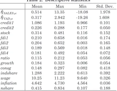
Table 2 presents a summary analysis of the main variables used in this paper, as well as reports the average provincial elasticity estimates from Eq. (1) when we use industrial value added instead of industrial sales.
The province elasticity estimates are denoted as
η ˆ
VAD pt andη ˆ
SALES pt , respectively.Table 2. Descriptive statistics
Mean Max Min Std. Dev.
η ˆ
SALES pt 0.514 13.35 -18.08 1.978η ˆ
VAD pt 0.317 2.942 -19.26 1.608credit1 1.086 1.193 0.966 0.101
credit2 0.226 0.288 0.177 0.050
stock 0.314 0.481 0.116 0.152
fdi1 0.210 0.658 0.016 0.174
fdi2 0.204 0.652 0.003 0.165
fdi3 0.189 0.569 0.018 0.148
fdi4 0.181 0.492 0.054 0.072
ratio 0.115 0.212 0.053 0.056
growth 0.184 0.323 0.006 0.054
consg 0.148 0.297 0.082 0.418
indshare 1.288 2.222 0.613 0.392
wage 10.25 11.23 9.640 0.326
inflation 4.642 4.730 4.564 0.036
nshare 0.415 0.834 0.107 0.188
3. Empirical analysis
3.1 The empirical specification
Endogeneity problem should be concerned when we take empirical test of the impact of financial development and FDI on investment allocation efficiency, because the financial development and FDI could promote the investment allocation efficiency while investment allocation efficiency would also bring more FDI and capital inflow. To reduce the endogeneity effects on parameter estimation, we adopt dynamic panel data model which includes the lag explained variable as follow:
η ˆ
pt= β0 +ρη ˆ
pt-1 + β1FDt + β2FDt * FDIpt + β3FDIpt + γ Xpt + δp+ εpt (2) wherep
represents the provinces;t
represents the year;η ˆ
pt is the measure of industrial sales elasticity of total fixed assets or industrial value added elasticity of total fixed assets;η ˆ
p,t-1 is the lagged item of theη ˆ
pt ; FD is the measure of financial development which includes credit1, credit2, and stock; FDIpt is the measure of FDI which includes fdi1, fdi2, fdi3, and fdi4;Xpt is a vector of provincial level control variables which contains growth, consg, indshare, wage, inflation, and nshare; δp is a time invariant province- specific intercept that captures omitted fixed effect; and εpt is the error term.
Eq. (2) contains the lagged dependent variable, which relates with the random disturbance term. If we use OLS to estimate the Eq. (2), it would yield biased and inconsistent estimates. Generally, dynamic panel data model with difference GMM (D-GMM) or system GMM (SYS -GMM) estimation method could solve the endogeneity problem validly. As a profit- driven capital, bank credit does not only affect the investment allocation
efficiency, but also is affected by the investment allocation efficiency, and the case of FDI is similar. In order to reduce the impact of this two- way feedback mechanism, we choose to use the system GMM method to estimate the dynamic panel data model, which effectively reflects the dynamic characters of investment behavior, reduces the impact of the two- way feedback mechanism on estimate results, and to a certain extent, obtains the consistent estimates.
3.2 The empirical results using industrial sales elasticity
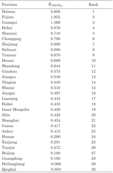
Table 3 reports the average sales elasticity of total fixed assets estimates from Eq.(1) between 2007 to 2012 of all 30 provinces. Theoretically, the coefficient of elasticity should be a positive number which is slightly less than 1. From table 2 we can clearly observe that most of the provinces are in the normal state, indicating that the investment is relatively stable. But there exist some questions with Hainan and Fujian, for which the growth rate of fixed asset investment is more than double of growth rate of sales.
The coefficient of Qinghai is also abnormal, but its fixed assets is reducing while the sales increasing, which suggesting that it is in normal situation.
Most of the elasticity coefficients have good fits.
Table 3. Estimates of the sales elasticity of total fixed assets
Province
η ˆ
SALESpt RankHainan 2.606 1
Fujian 1.955 2
Guangxi 1.366 3
Hebei 0.876 4
Shannxi 0.710 5
Chongqing 0.706 6
Zhejiang 0.699 7
Sichuan 0.688 8
Yunnan 0.670 9
Henan 0.669 10
Shandong 0.644 11
Guizhou 0.575 12
Jiangsu 0.549 13
Ningxia 0.530 14
Shanxi 0.510 15
Jiangxi 0.497 16
Liaoning 0.445 17
Hubei 0.432 18
Inner Mongolia 0.429 19
Jilin 0.428 20
Shanghai 0.424 21
Gansu 0.417 22
Anhui 0.413 23
Hunan 0.290 24
Xinjiang 0.281 25
Tianjin 0.272 26
Beijing 0.180 27
Guangdong 0.108 28
Heilongjiang -0.066 29
Qinghai -0.883 30
Note: Estimates of the elasticity from Eq.(1)
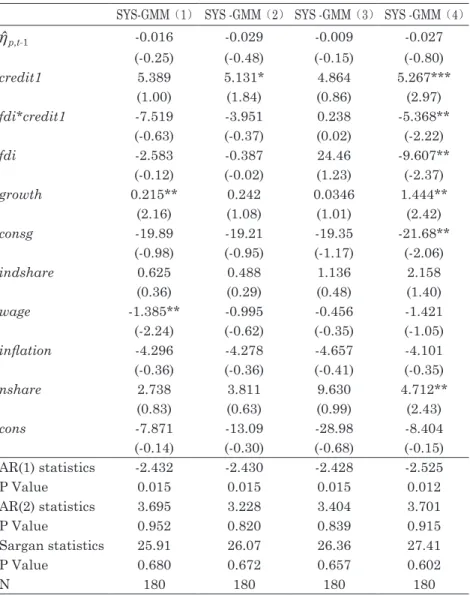
We introduce the first-order lag consequent of explained variable in dynamic panel data model, setting financial development variables (credit1,
credit2, stock), FDI variables (fdi1, fdi2, fdi3, fdi4) and their interaction terms, area economic growth indicator growth as endogenous variable, with other control variables being exogenous variables. Estimation results of the dynamic panel data model with system generalized method of moments (SYS-GMM) are shown in Table 4. In SYS-GMM (1) - (4), fdi1, fdi2, fdi3, fdi4 are used as FDI variable, respectively. In panel A, the financial development indicator is credit1, while the indicators of financial development in panel B and panel C are credit2 and stock, respectively.
The interaction between financial development and FDI is also examined.
Usually we could determine whether the GMM method is applicable through the test of autocorrelation of disturbance item in dynamic panel data model. The specific approach is to test the autocorrelation of the first-order and second-order difference of disturbance item under the null hypothesis “disturbance item does not exist correlation” in the original level equation, and then we could gain two statistics for AR(1) and AR(2).
If AR(1) is significant while AR(2) is not, then it indicates that the null hypothesis cannot be rejected. At the same time, the Sargan statistic is used to test the validity of instrument variables in GMM estimation (Zhao, 2014). Estimation results in Table 4 show that, the AR(1)s of all the model are significant at 5% significant level, and AR(2)s are insignificant.
Sargan statistics show that we cannot reject the null hypothesis that the instrumental variables are valid, indicating that the model is reasonable.
We use robust standard errors when estimating the model, in order to ensure the validity of the parameter estimation results.
In column (1)-(4) of Panel A, we regress
η ˆ
SALES pt on indicator of financial development indicator credit1, and fdi1, fdi2, fdi3, fdi4 respectively.The results display that financial development has positive effect on
the investment allocation efficiency, for the coefficients of credit1 are all positive. However, we do find the coefficients of FDI are negative, meaning that too much FDI will bring negative impact on the long-term allocation of capital. After further analysis, we think that FDI has the crowding out effect to the domestic capital. The coefficients of interactive terms between financial development index and FDI are also negative which indicate that FDI can weaken the positive effect of financial development on investment allocation.
In column (1)-(4) of Panel B, we use credit2 (measured by domestic credit to private sector) as the indicator of financial development. The results are similar to those in Panel A. The four coefficients of credit2 are all positive and insignificant, meaning that the bank credit flowing to private sector does not affect the investment allocation efficiency, and China's bank credit market could not effectively allocate resources for private economy. Coefficients of FDI are significantly negative, indicating that the increase of flow and stock of FDI both have a negative impact on the investment allocation efficiency in China. The coefficients of interactive terms between financial development and FDI are also negative, which show that the joint increase of FDI and domestic credit may further reduce the investment allocation efficiency.
In column (1)-(4) of Panel C, we use stock (measured by total value of stocks traded) as financial development indicator. The coefficients of stock are significantly negative when we regress dependent variable on fdi2, meaning that the ratio between the market value of stocks traded and GDP has negative effect on investment allocation efficiency. Coefficients of FDI are all negative but insignificant. However, the coefficients of interaction terms between financial development and FDI are significantly negative,
which implies that there is a competition and crowding out effect between the stock market and FDI. In fact, both of them are capital searching for high return, and the competition between them is relatively fierce.
Overall, all the coefficients of lagged dependent variables
η ˆ
p,t-1 are insignificant, meaning that there is no continuity of investment allocation efficiency, i.e., the efficiency of the current period is not affected by the efficiency of previous year to a large extent. Most of the FDI coefficients are insignificant, we believe that the low ratio of FDI in total investment is one reason for this result.Table 4. Effects of financial development and FDI on sales elasticity of total fixed assets
Panel A
SYS-GMM(1) SYS -GMM(2)SYS -GMM(3)SYS -GMM(4)
η ˆ
p,t-1 -0.016 -0.029 -0.009 -0.027(-0.25) (-0.48) (-0.15) (-0.80)
credit1 5.389 5.131* 4.864 5.267***
(1.00) (1.84) (0.86) (2.97)
fdi*credit1 -7.519 -3.951 0.238 -5.368**
(-0.63) (-0.37) (0.02) (-2.22)
fdi -2.583 -0.387 24.46 -9.607**
(-0.12) (-0.02) (1.23) (-2.37)
growth 0.215** 0.242 0.0346 1.444**
(2.16) (1.08) (1.01) (2.42)
consg -19.89 -19.21 -19.35 -21.68**
(-0.98) (-0.95) (-1.17) (-2.06)
indshare 0.625 0.488 1.136 2.158
(0.36) (0.29) (0.48) (1.40)
wage -1.385** -0.995 -0.456 -1.421
(-2.24) (-0.62) (-0.35) (-1.05)
inflation -4.296 -4.278 -4.657 -4.101
(-0.36) (-0.36) (-0.41) (-0.35)
nshare 2.738 3.811 9.630 4.712**
(0.83) (0.63) (0.99) (2.43)
cons -7.871 -13.09 -28.98 -8.404
(-0.14) (-0.30) (-0.68) (-0.15)
AR(1) statistics P Value
-2.432 0.015
-2.430 0.015
-2.428 0.015
-2.525 0.012 AR(2) statistics
P Value
3.695 0.952
3.228 0.820
3.404 0.839
3.701 0.915 Sargan statistics
P Value
25.91 0.680
26.07 0.672
26.36 0.657
27.41 0.602
N 180 180 180 180
Panel B
SYS-GMM(1) SYS -GMM(2)SYS -GMM(3)SYS -GMM(4)
η ˆ
p,t-1 -0.044 -0.006 -0.036 -0.015(-0.94) (-0.29) (-0.83) (-0.39)
credit2 8.779 7.092 7.539 11.79
(1.17) (0.80) (0.78) (1.18)
fdi*credit2 -26.20** -15.01** -14.77 -29.82**
(-2.18) (-2.22) (-0.69) (-2.35)
fdi -6.686** -1.102 -26.04*** -10.70**
(-2.29) (-0.10) (-2.72) (-2.42)
growth 0.405** 0.640 0.347 0.937**
(2.15) (0.17) (0.09) (2.24)
consg -20.09 -19.97 -20.36** -21.81
(-0.95) (-0.96) (-2.19) (-1.04)
indshare 0.319 0.413 0.945 2.279
(0.19) (0.24) (0.41) (1.19)
wage -0.730 -0.283 0.295 -1.319
(-0.52) (-0.16) (0.18) (-0.83)
inflation -0.360 -0.706 -0.966 -0.245
(0.05) (-0.07) (-0.11) (0.03)
nshare 3.134 4.670 10.24 4.200
(0.99) (0.73) (1.05) (1.50)
cons 8.303 6.600 -6.419 12.08
(0.25) (0.23) (-0.24) (0.35)
AR(1) statistics P Value
-2.515 0.013
-2.504 0.013
-2.510 0.013
-2.479 0.014 AR(2) statistics
P Value
4.021 0.983
3.665 0.948
3.942 0.967
3.505 0.917 Sargan statistics
P Value
25.65 0.693
24.75 0.737
24.45 0.751
26.41 0.654
N 180 180 180 180
Panel C
SYS-GMM(1) SYS -GMM(2)SYS -GMM(3)SYS -GMM(4)
η ˆ
p,t-1 -0.031 -0.019 -0.010 -0.026(-0.25) (-0.48) (-0.15) (-0.80)
stock -1.542 -2.598** -3.505 1.394
(-0.43) (-2.16) (-0.99) (0.86)
fdi*stock -0.662 4.252 2.758 -16.58**
(-0.06) (0.70) (0.24) (-2.30)
fdi -8.602 -6.522 26.35 -10.27
(-0.35) (-0.69) (1.74) (-0.41)
growth 1.525*** 0.930 2.406 2.840**
(2.58) (0.37) (0.75) (2.11)
consg -21.43 -20.25 -20.59** -21.41
(-0.95) (-0.92) (-2.15) (-0.98)
indshare 0.832 0.435 1.179 1.869
(0.46) (0.24) (0.49) (0.98)
wage 0.576 1.048 2.515** 0.498
(0.29) (1.06) (2.46) (0.25)
inflation -6.416 -6.928 -11.34** -6.577
(-1.12) (-0.88) (-2.17) (-1.09)
nshare 3.517 3.495 11.16 4.137
(1.03) (0.49) (1.08) (1.63)
cons 27.08 24.61 19.79 27.14
(0.87) (0.80) (0.68) (0.84)
AR(1) statistics P Value
-2.463 0.014
-2.426 0.015
-2.454 0.014
-2.562 0.012 AR(2) statistics
P Value
3.165 0.869
2.301 0.763
2.471 0.786
3.477 0.920 Sargan
P Value
25.28 0.712
21.12 0.884
26.09 0.671
18.60 0.948
N 180 180 180 180
t statistics in parentheses, * p < 0.1, ** p < 0.05, *** p < 0.01
Of the six additional variables, the coefficients of growth, the growth rate of provincial real gross domestic product are positive, suggesting
that increases in GDP can lead to growth in long term investment. The coefficients of inflation, the log of annual price indices for investment in fixed assets by region, are negative, indicating that the rapid rise of cost would bring down the investment in fixed assets. The coefficients of wage, the provincial average wage of staff and workers, are different within different situation. In panel A, the coefficients are all negative, but they are all positive in panel C. The coefficients of consg, the ratio of provincial government consumption to provincial gross domestic product, are always negative but most of them are insignificant. The coefficients of indshare, the proportion of the ratio of provincial gross industry output value to provincial gross domestic product, are always insignificantly positive. The coefficients of nshare, the ratio of gross industry output value of state-owned and state-holding industrial enterprises to gross industry output value of industrial enterprises above designated size, are always insignificantly positive. Wurgler (2000) claims that the efficiency of capital allocation is negatively correlated with the extent of state ownership in the economy, which is not supported by our findings.
3.3 The empirical results using industrial velus added elasticity Wurgler (2000) argues that growth in value added reflects investment opportunities. In this part, we use industrial value added instead of industry sales to estimate the elasticity of industry investment from Eq.(1).
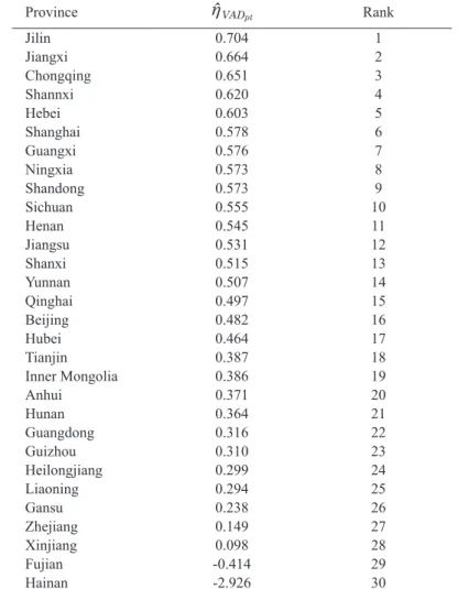
Table 5 reports the average industrial value-added elasticity of total fixed assets in 30 regions. According to the above, the coefficient of elasticity should be a positive number. From Table 5, we can find that most of the industrial value added elasticity of total fixed assets are range from 0.3- 0.8, which is a normal range. The coefficients of elasticity are negative in
Hainan and Fujian, meaning that the investment allocation efficiency of these two provinces is low and should be optimized timely.
Table 5. Estimates of the industrial value added elasticity of total fixed assets
Province
η ˆ
VADpt RankJilin 0.704 1
Jiangxi 0.664 2
Chongqing 0.651 3
Shannxi 0.620 4
Hebei 0.603 5
Shanghai 0.578 6
Guangxi 0.576 7
Ningxia 0.573 8
Shandong 0.573 9
Sichuan 0.555 10
Henan 0.545 11
Jiangsu 0.531 12
Shanxi 0.515 13
Yunnan 0.507 14
Qinghai 0.497 15
Beijing 0.482 16
Hubei 0.464 17
Tianjin 0.387 18
Inner Mongolia 0.386 19
Anhui 0.371 20
Hunan 0.364 21
Guangdong 0.316 22
Guizhou 0.310 23
Heilongjiang 0.299 24
Liaoning 0.294 25
Gansu 0.238 26
Zhejiang 0.149 27
Xinjiang 0.098 28
Fujian -0.414 29
Hainan -2.926 30
Note: Estimates of the elasticity are obtained from Eq.(1)
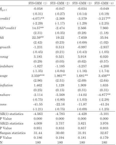
We now provide the econometric evidence on the effect of financial development and FDI on the industrial value added elasticity of total fixed assets,
η ˆ
VAD pt . Similarly to section 3.2, here we take credit1, credit2, and stock as indicators of financial development. The regression results are reported in Table 6.In column (1)-(4) of Panel A, we regress
η ˆ
VAD pt on indicator of financial development, credit1, and fdi1, fdi2, fdi3, fdi4, respectively. These results are different from the above results significantly. All of the coefficients of credit1 are negative, and results in column (1) and (4) are statistically significant at the 5% level, indicating a negative relationship between credit loan and investment efficiency. The coefficients of FDI in column (1) is significantly positive, suggesting that higher ratio of FDI market share contributes to investment in fixed assets. In column (1), the coefficient of interactive terms between financial development index credit1 and FDI is positive. The threshold value of FDI is 0.279, and the mean value is 0.21 (as shown in Table 2), suggesting that FDI was below the minimum threshold value to fully promote the marginal effects of domestic bank loan.In column (1) and (4) of Panel B, two coefficients of credit2 are significantly negative. In column (1), the coefficient of credit2 is -8.110; the coefficient of interactive terms between financial development index credit2 and FDI is 41.92. Hence, the threshold value of FDI is 0.193, smaller than the mean value 0.21, indicating that FDI reached the minimum threshold value to fully promote the marginal effects of domestic loans to the private sector.
Unlike results in Table 4, column (1)-(4) of Panel C in Table 6 show significantly positive coefficients of stock, suggesting positive effects of stock on investment allocation. In column (1) and (2), coefficients of FDI are
significantly positive, indicating that increases in FDI ratio can improve the efficiency of fixed assets investment. In column (4), the coefficient of interactive terms between stock and FDI is significantly positive, showing that stock market activities along with FDI encourage investment in fixed assets.
The coefficients of interaction terms between financial development index and FDI show that there is no competition and crowding out effect between financial development and FDI when we take industrial value- added elasticity of total fixed assets to indicate the investment allocation efficiency.
Table 6. Effects of financial development and FDI on industrial value added elasticity of total fixed assets
Panel A
SYS-GMM(1) SYS -GMM(2)SYS -GMM(3)SYS -GMM(4)
η ˆ
p,t-1 -0.058 -0.047 -0.034 -0.049(-0.31) (-0.27) (-0.14) (-0.19)
credit1 -4.071** -2.368 -3.379 -3.217**
(-2.29) (-1.17) (-1.29) (-2.25)
fdi*credit1 14.57** -2.474 2.566 7.960
(2.31) (-0.35) (0.28) (1.18)
fdi 22.59** 19.22 -7.659 35.94
(2.42) (0.23) (-0.68) (1.02)
growth -1.231 0.513 -0.997 -2.937
(-0.45) (0.21) (-0.43) (-1.05)
consg 3.185 0.521 5.918 6.020
(0.29) (0.05) (0.62) (0.57)
indshare -1.827 -1.185 -3.257 -4.200
(-1.35) (-0.84) (-1.16) (-1.74)
wage 3.359*** 1.961** 1.681** 3.456**
(2.96) (2.51) (2.69) (2.64)
inflation 1.462 1.128 1.909 1.635
(0.25) (0.15) (0.31) (0.31)
nshare -2.114 -5.568 -14.02 -4.877**
(-0.75) (-0.80) (-1.03) (-2.28)
cons -41.55 -22.16 -11.87 -41.24
(-1.21) (-0.75) (-0.69) (-1.25)
AR(1) statistics -4.563 -4.783 -4.428 -5.101
P Value 0.000 0.000 0.000 0.000
AR(2) statistics 4.009 3.757 3.821 3.976
P Value 0.951 0.833 0.857 0.933
Sargan statistics 31.44 30.60 31.91 32.67
P Value 0.186 0.194 0.181 0.179
N 180 180 180 180
Panel B
SYS-GMM(1) SYS -GMM(2)SYS -GMM(3)SYS -GMM(4)
η ˆ
p,t-1 -0.083 -0.036 -0.055 -0.089(-0.41) (-0.25) (-0.17) (-0.17)
credit2 -8.110** -2.134 -6.407 -10.48**
(-2.26) (-0.44) (-0.94) (-2.22)
fdi*credit2 41.92** 2.888 21.13 39.43
(2.27) (0.27) (0.76) (1.84)
fdi 30.69 15.50 -7.737 36.82
(1.44) (1.01) (-1.00) (1.04)
growth -0.630 0.349 -0.668 -2.485
(-0.23) (0.12) (-0.27) (-0.84)
consg 2.947 1.267 6.617 5.483
(0.26) (0.12) (0.68) (0.51)
indshare -1.500 -1.178 -3.077 -4.220
(-1.28) (-0.82) (-1.19) (-1.76)
wage 2.819*** 1.242 1.134 3.618**
(2.56) (0.92) (1.13) (2.29)
inflation 2.234 5.274 5.157 2.608
(0.53) (0.61) (0.81) (0.61)
nshare -2.646 -6.548 -14.59** -3.890
(-0.95) (-0.86) (-2.27) (-1.16)
cons -42.82 -35.73 -24.07 -49.18
(-1.73) (-1.28) (-1.57) (-1.77)
AR(1) statistics -4.717 -5.012 -4.790 -5.434
P Value 0.000 0.000 0.000 0.000
AR(2) statistics 4.013 3.568 3.786 3.946
P Value 0.952 0.820 0.839 0.915
Sargan statistics 30.62 31.90 31.21 31.92
P Value 0.193 0.182 0.187 0.181
N 180 180 180 180
Panel C
SYS-GMM(1) SYS -GMM(2)SYS -GMM(3)SYS -GMM(4)
η ˆ
p,t-1 -0.081 -0.050 -0.061 -0.099(-0.21) (-0.13) (-0.34) (-0.51)
stock 0.253 3.066 2.679** 0.489
(0.15) (1.68) (2.42) (0.38)
fdi*stock 9.171 -1.850 5.474 9.890**
(0.95) (-0.47) (0.47) (2.37)
fdi 33.03** 16.34** -8.614 3.75
(2.43) (2.49) (-1.24) (1.38)
growth -2.769 -1.557 -3.842 -3.163
(-1.02) (-0.51) (-1.13) (-1.15)
consg 3.998 1.574 6.824 4.346
(0.35) (0.14) (0.68) (0.39)
indshare -2.044 -1.285 -3.251 -2.921
(-1.26) (-0.82) (-1.13) (-1.29)
wage 2.011 -0.175 -1.005 2.096
(1.60) (-0.16) (-0.80) (1.54)
inflation 8.993* 12.98 16.63* 9.305*
(2.00) (1.20) (2.49) (2.02)
nshare -3.097 -6.809 -15.75* -2.808
(-0.90) (-0.88) (-2.29) (-0.85)
cons -65.82** -57.78 -55.70 -67.53**
(-2.11) (-1.51) (-1.80) (-2.10)
AR(1) statistics -5.023 -5.167 -4.890 -5.876
P Value 0.000 0.000 0.000 0.000
AR(2) statistics 3.657 3.951 3.814 4.091
P Value 0.814 0.877 0.852 0.941
Sargan statistics 30.78 32.24 31.94 31.47
P Value 0.191 0.173 0.180 0.185
N 180 180 180 180
t statistics in parentheses * p < 0.1, ** p < 0.05, *** p < 0.01
Among the control variable, the coefficients of wage are significantly positive in Panel A as well as in column (1) and (4) of Panel B, suggesting
that increases in wage lead fixed investment to industries with higher growth rates. In Table 6, coefficients of nshare are significantly negative, confirming with the findings of Wurgler (2005) in the sense that the large state-owned share in Chinese economy prevents capital to be allocated to industries with a rapid growth. The coefficients of other variables such as growth and inflation are insignificant, suggesting mild effects on investment allocation that aims at increasing industrial added value.
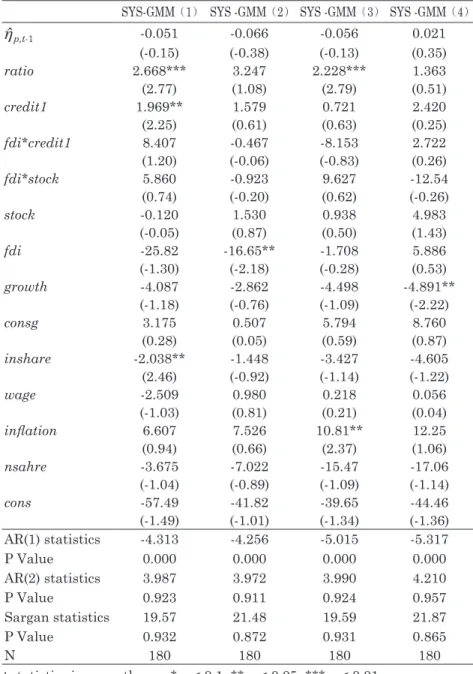
4. The effect of financial structure on allocation of investment Besides studying the effects of FDI and financial development on efficiency of investment allocation, we investigate how financial structure affects investment efficiency. Previous debate on financial structure are mainly conducted from four aspects: bank, market, financial services, and law. The bank-based view highlights the positive role of banks that banks are more effective in providing external resources to investment activities (Allen & Gale, 2004). The market-based view stresses both the positive role of markets and the comparative advantages of markets over banks in effectively allocating capital. They emphasize that powerful banks frequently stymie innovation by extracting informational rents and banks have an inherent bias toward conservative investments (Morck et al., 1999;
La Porta et al., 2002; Stiglitz, 1985). The financial services view argues that the bank-based versus market-based debate is not important. It is financial services themselves that are by far more important, than the form of their delivery (Luintel et al., 2008). The law and finance view emphasizes the role of the legal system which protects outside investors by enforcing contracts effectively and boosts financial development and thereby facilitates external financing and efficient capital allocation (La Porta et al,2000).
In this part, we use ratio as the measure of financial structure, the variable is defined as the proportion of domestic stock issuance to the increased amount of bank loan, to examine its impact on the efficiency of capital allocation. The econometric evidence on the effect of financial structure on the elasticity estimates of industry investment to industry sales,
η ˆ
SALES pt , arereported in Table 7. In column (1)-(4), we regress
η ˆ
SALES pt on indicators of fdi1, fdi2, fdi3, fdi4, respectively, and on indicators of financial development credit1, stock with their interactive terms with FDI, as well as other control variables. The coefficients of ratio are significantly positive which implies that the ratio of domestic raised capital in stock market to amount of loan of bank promotes the effect in investment allocation as it increases.It seems that our results are in favor of market-based view. Although substantial proportions of the shares of many listed firms are owned by the state and they cannot be traded freely in Chinese stock market, as the proportion of private economy to the overall economy gradually rise, the function of capital allocation of stock market will be strengthened.
Table 7. The effect of financial structure on allocation of investment SYS-GMM(1) SYS -GMM(2)SYS -GMM(3)SYS -GMM(4)
η ˆ
p,t-1 -0.051 -0.066 -0.056 0.021(-0.15) (-0.38) (-0.13) (0.35)
ratio 2.668*** 3.247 2.228*** 1.363
(2.77) (1.08) (2.79) (0.51)
credit1 1.969** 1.579 0.721 2.420
(2.25) (0.61) (0.63) (0.25)
fdi*credit1 8.407 -0.467 -8.153 2.722
(1.20) (-0.06) (-0.83) (0.26)
fdi*stock 5.860 -0.923 9.627 -12.54
(0.74) (-0.20) (0.62) (-0.26)
stock -0.120 1.530 0.938 4.983
(-0.05) (0.87) (0.50) (1.43)
fdi -25.82 -16.65** -1.708 5.886
(-1.30) (-2.18) (-0.28) (0.53)
growth -4.087 -2.862 -4.498 -4.891**
(-1.18) (-0.76) (-1.09) (-2.22)
consg 3.175 0.507 5.794 8.760
(0.28) (0.05) (0.59) (0.87)
inshare -2.038** -1.448 -3.427 -4.605
(2.46) (-0.92) (-1.14) (-1.22)
wage -2.509 0.980 0.218 0.056
(-1.03) (0.81) (0.21) (0.04)
inflation 6.607 7.526 10.81** 12.25
(0.94) (0.66) (2.37) (1.06)
nsahre -3.675 -7.022 -15.47 -17.06
(-1.04) (-0.89) (-1.09) (-1.14)
cons -57.49 -41.82 -39.65 -44.46
(-1.49) (-1.01) (-1.34) (-1.36)
AR(1) statistics -4.313 -4.256 -5.015 -5.317
P Value 0.000 0.000 0.000 0.000
AR(2) statistics 3.987 3.972 3.990 4.210
P Value 0.923 0.911 0.924 0.957
Sargan statistics 19.57 21.48 19.59 21.87
P Value 0.932 0.872 0.931 0.865
N 180 180 180 180
t statistics in parentheses * p < 0.1, ** p < 0.05, *** p < 0.01
5. Conclusions
China's proportion of fixed investment in GDP is much higher than those in the developed countries, which makes the conventional indicator of investment allocation efficiency less applicable for Chinese economic data.
After comparing various economic indicators, we consider using industrial sales to calculate the investment allocation efficiency to effectively describe the current status of investment. Therefore, using China’s provincial panel data set containing 17 industries from 2006 to 2012, we set two investment allocation efficiency indicators, the industrial sales elasticity of total fixed assets and the industrial value-added elasticity of total fixed assets, respectively, and then assess the effect of financial development and foreign direct investment on the two indicators. When using the industrial sales elasticity of total fixed assets to indicate investment allocation efficiency, we find that the total bank credit improves the investment allocation efficiency significantly, while the bank credit to the private sector only influences the investment allocation efficiency mildly. Unlike most of existing literature, we claim that FDI and stock market play opposite roles in promoting investment. There exist great competition and crowding out between bank credit, private sector bank credit, stock market scale and FDI; despite the crowding out effect, bank credit improves the investment allocation efficiency significantly. As the substitution effect of China's securities market on bank credit gradually gets stronger, investment allocation efficiency has been improved to a larger extent. Contradictory results are obtained by using industrial value-added elasticity of total fixed assets as the efficiency indicator. In particular, total domestic bank credit and bank credit to the private sector both have negative effect on the investment allocation efficiency, but FDI could promote the investment
allocation efficiency to a certain extent. Furthermore, FDI is below the minimum threshold value to make the total domestic bank loan have a positive marginal effect, but it reaches the minimum threshold value to make domestic loans to the private sector have a positive marginal effect.
Stock market also has a positive effect on investment allocation efficiency.
Anyways, there is no competition and crowding out effect between financial development and FDI, when we take industrial value-added elasticity of total fixed assets to indicate the investment allocation efficiency. The effect of all the other control variables on investment allocation also root in distinguishing between the two elasticities.
In sum, China's economy is mainly spurred by investment, and investment has a very obvious sales-driven phenomenon. We find that significant differences exist between the two investment allocation efficiency indicators calculated by industrial sales and industrial added value, and so are their influence factors and path. Therefore, policy makers should make investment decisions based on the economic status, development plan and, select the optimum investment scheme, and then transform the sales-driven investment into industrial added value driven investment gradually, in order to achieve benefit maximization.
References
Allen, F. and D. Gale, 2004, Financial intermediaries and markets, Econometrica, 72, pp.1023-1061.
Alfaro, L., A. Chanda and S. Kalemli-Ozcan, 2004, FDI and economic growth: the role of local financial markets, Journal of International Economics, 64, pp.89–112.
Alfaro, L., A. Chanda, S. Kalemli-Ozcan and S. Sayek, 2010, Does foreign direct investment promote growth? Exploring the role of financial markets on linkages, Journal of Development Economics, 91, pp.242-256.
Aurangzeb, Z and Stengos, T, 2014, The role of Foreign Direct Investment (FDI) in a dualistic growth framework: A smooth coefficient semi-parametric approach, Borsa
Istanbul Review, 14, pp.133–144.
Beck, T and Levine, R, 2002, Industry growth and capital allocation: does having a market- or bank-based system matter? Journal of Financial Economics, 64,pp 147-180.
Calderon, C. and L. Liu, 2003, The direction of causality between financial development and economic growth, Journal of Development Economics, 72, pp.321– 334.
Chen, J. and Y. Sheng, 2008, An empirical study on FDI international knowledge spillovers and regional economic development in China, Economic Research Journal, 43, pp.39–49.
Christopoulos, D. K. and E. G. Tsionas, 2004, Financial development and economic growth: evidence from panel unit root and cointegration tests, Journal of Development Economics, 73, pp.55– 74.
Galindo, A., F. Schiantarelli and A. Weiss, 2007, Does financial liberalization improve the allocation of investment? Micro-evidence from developing countries, Journal of Development Economics, 83, pp.562–587.
Harrison, A. E. and M. S. McMillan, 2003, Does direct foreign investment affect domestic credit constraints?, Journal of International Economics, 61, pp.73–100.
Islam, S. S. and A. Mozumdar, 2006, Financial market development and the importance of internal cash: Evidence from international data, Journal of Banking & Finance, 31, pp.641–658.
Lee, C. and Chang. C. 2009, FDI, financial development, and economic growth:
international evidence, Journal of Applied Economics, 12, pp.249–271.
Li.Q.,Q.Zhao, J.Li,c.Jiang, 2010, Foreign direct investment, financial development and regional capital allocation efficiency-Evidence from provincial industry data, Journal of financial research, No3, pp80-97.
Liu, S., 2008, International trade, FDI and declines in China’s TFP, Journal of Quantitative & Technical Economics, 25, pp.28–39.
Luintel, K. B., M. Khan, P. Arestis, and K. Theodoridis, 2008, Financial structure and economic growth, Journal of Development Economics, 86, pp.181–200.
Morck, R. and M. Nakamura, 1999. Banks and corporate control in Japan. Journal of Finance 54, 319–340.
Morck,R , Yavuz,D and Yeung,B, 2011, Banking system control, capital allocation, and economy performance, Journal of Financial Economics, 100,pp 264–283.
Ndikumana, L., 2005, Financial development, financial structure, and domestic investment: International evidence, Journal of International Money and Finance, 24, pp.651-673.
Pang, J. and H. Wu, 2009, Financial markets, financial dependence, and the allocation of capital, Journal of Banking & Finance, 33, pp.810–818.
Rioja, F. and N. Valev, 2004, Does one size fit all? A reexamination of the finance and growth relationship, Journal of Development Economics, 74, pp.429– 447.
Stiglitz, J.E., 1985. Credit markets and the control of capital. Journal of Money Credit and
Banking 17, 133–152.
Sun, L., 2008, Financial development, FDI and economic growth, Journal of Quantitative
&Technical Economics, 25, pp.3-14.
Taboada, A.G., 2011, The impact of changes in bank ownership structure on the allocation of capital: International evidence, Journal of Banking & Finance, 35, 2528–2543 Wang, L. and T. Qin, 2007, An Analysis on the Conditions of FDI Productivity Spillovers
in Chinese Manufacturing Sector, China Economic Quarterly, 6, pp.171-184.
Wang, L. Wu and Y. Yang, 2009, Does the stock market affect firm investment in China? A price informativeness perspective, Journal of Banking & Finance, 33,pp. 53–62.
Wang, Y. FDI spillovers,2006, financial market and economic growth, Journal of Quantitative & Technical Economics, 23 , pp.59–68.
Wurgler, J., 2000, Financial markets and the allocation of capital, Journal of Financial Economics, 58, pp.187-214.
Xie, J., 2006, Technical spillovers if foreign direct investment in China, China Economic Quarterly, 5 , pp.1109–1128.
Yang, X. and Y. Lai, 2006, FDI and technology spillovers, Journal of Quantitative &
Technical Economics, 23 , pp.72–81.
Yao, S., G. Feng, and K. Wei, 2006, Economic growth in the presence of FDI, Economic Research Journal, 41, pp.35–46.
Zhao, Q. and C. Zhang, 2006, Technology spillover effects of FDI and economy growth, Journal of Quantitative & Technical Economics, 23, pp.111–120.
Zhao, G., 2014, Advanced Econometrics: Methods and Applications, Renmin University of China Press.
提出年月日:2016 年 5 月 16 日