Strategy-proofness and Efficiency with Nonquasi-linear Preferences: A Characterization of Minimum Price Walrasian Rule

Discussion Paper No. 852

STRATEGY-PROOFNESS AND EFFICIENCY WITH NONQUASI-LINEAR PREFERENCES:

A CHARACTERIZATION

OF MINIMUM PRICE WALRASIAN RULE

Shuhei Morimoto Shigehiro Serizawa

August 2012

The Institute of Social and Economic Research Osaka University

6-1 Mihogaoka, Ibaraki, Osaka 567-0047, Japan

Strategy-proofness and Efficiency with

Nonquasi-linear Preferences: A Characterization of Minimum Price Walrasian Rule ^∗

Shuhei Morimoto

and Shigehiro Serizawa

August 10, 2012

Abstract

We consider the problems of allocating several heterogeneous objects owned by gov- ernments to a group of agents and how much agents should pay. Each agent receives at most one object and has nonquasi-linear preferences. Nonquasi-linear preferences de- scribe environments in which large-scale payments influence agents’ abilities to utilize objects or derive benefits from them. The “minimum price Walrasian (MPW) rule” is the rule that assigns a minimum price Walrasian equilibrium allocation to each pref- erence profile. We establish that the MPW rule is the unique rule that satisfies the desirable properties of

on the domain that includes nonquasi-linear preferences. This result does not only recommend the MPW rule based on those desirable properties, but also suggest that governments cannot improve upon the MPW rule once they consider them essential. Since the outcome of the MPW rule coincides with that of the simulta- neous ascending (SA) auction, our result explains the pervasive use of the SA auction.

Keywords:

minimum price Walrasian equilibrium, simultaneous ascending auction, strategy-proofness, efficiency, heterogeneous objects, nonquasi-linear preferences

D44, D71, D61, D82

∗A preliminary version of this article was presented at the conference honoring Salvador Barber`a’s 65th birthday at the Universitat Aut`onoma de Barcelona in June 2011; Frontiers of Market Design at Ascona, Switzerland in May 2012; and the APET 13th annual conference in Taipei, Taiwan in June 2012. We thank participants at those conferences for their valuable comments. We are also grateful to seminar participants at Hitotsubashi, Keio, Kobe, Kyoto, Tohoku, and Waseda universities for their helpful comments. We specially thank Professors A. Kajii, D. Mishra, S. Ohseto, J. Schummer, W. Thomson, and J. Wako for their detailed comments. Remaining errors are ours.

†Institute of Social and Economic Research, Osaka University, 6-1, Mihogaoka, Ibaraki, 567-0047, Japan.

E-mail: [email protected]

‡Institute of Social and Economic Research, Osaka University, 6-1, Mihogaoka, Ibaraki, 567-0047, Japan.

E-mail: [email protected]

1 Introduction

Purpose. Since the 1990s, governments in numerous countries have conducted auctions to allocates a variety of heterogeneous objects or assets including spectrum rights, vehicle ownership licenses, and lands, etc. Although auction revenues sometimes amount to even as large as government annual budgets, the announced goals of many government auctions are rather to allocate objects “efficiently”, i.e., to agents who make the most use of them or benefit most from them.

Agents making more use of objects or benefiting more are willing to pay higher prices for them, and thus would have more chances to win the objects in auctions.

However, large-scale auction payments would influence agents’ abilities to utilize objects or benefit from them, thereby complicating efficient allocation. This article analyzes rules that allocate auctioned objects efficiently even when payments are so large that it impairs agents’

abilities to utilize them or realize their benefits. We ask what types of allocation rules can allocate objects efficiently in such environments.

Main Result. An allocation rule (or simply a rule ) is a function that assigns to each agents’ preference profile an allocation, which consists of an assignment of objects and agents’

payments. Each agent is permitted to receive one object at the most. The domain of rules is the class of agents’ preference profiles. It is well-known that in this model, there is a minimum price Walrasian equilibrium,

and that its allocation coincides with the outcome of the simultaneous ascending (SA) auction.

We focus on the rule that assigns a minimum price Walrasian equilibrium allocation to each preference profile. We refer to this rule as the

“minimum price Walrasian (MPW) rule”.

The MPW rule satisfies four desirable properties. The first is Pareto-efficiency. An allocation is Pareto-efficient if no agent can be better off without making other agents worse off or reducing a government’s revenue.

Note that Pareto-efficiency is evaluated based on agents’ preferences. Thus, a Pareto-efficient allocation cannot be chosen without information about agents’ preferences. Since preferences are private information, agents have incentives to behave strategically to influence the final outcome in their favor. Strategy-proofness is an incentive-compatibility property, which gives a strong incentive for each agent to reveal his true preferences. It says that in the normal form game induced by the rule, it is a (weakly) dominant strategy for each agent to reveal his true preference. The MPW rule satisfies strategy-proofness,

and chooses a Pareto-efficient allocation corresponding to the revealed preferences.

Third property is individual rationality, that induces agents’s voluntary participation.

The MPW rule never assigns an allocation that makes an agent worse off than he would be if he had received no object and paid nothing. Fourth is nonnegative payment. Under the MPW rule, agents’ payments are always nonnegative, that is, governments never subsidize agents.

The primary conclusion of this article is that only the minimum price Walrasian rule sat-

1For example, frequency auctions in the United States were introduced to promote “efficient and intensive use of the electromagnetic spectrum”. See McAfee and McMillan (1996, p.160).

2See Demange and Gale (1985).

3For example, see Demange, Gale, and Sotomayor (1986).

4In our auction model,Pareto-efficiency is defined by taking government revenue into account.

5In addition, the MPW rule satisfies group strategy-proofness, i.e., by misrepresenting their preferences, no group of agents should obtain assignments that they prefer.

isfies strategy-proofness, Pareto-efficiency, individual rationality, and nonnegative payment in environments where large-scale payments influence agents’ abilities to utilize the objects or enjoy their benefits(Theorem 5.1). This result does not only recommend the MPW rule based on the four desirable properties, but also implies that no other rules are available options once governments consider the four properties as essential. Since the outcome of the MPW rule coincides with that of the SA auction, the result also supports SA auctions adopted by many governments.

Novelties and technical difficulties. Holmstr¨ om (1979) establishes a fundamental result relating to our question that applies when agents’ benefits from auctioned objects are not influenced by their payments, i.e., agents have “quasi-linear” preferences. He assumes that the domain includes only quasi-linear preference, and shows that only the Vickrey–

Clarke–Groves type (VCG)

allocation rules satisfy strategy-proofness and Pareto-efficiency.

Preferences are approximately quasi-linear if payments are sufficiently low. However, quasi- linearity is not an appropriate assumption for large-scale auctions. Excessive payment for the auctioned objects may damage bidders’ budgets and render effective use of the objects impossible. In fact, in spectrum license auctions and vehicle ownership license auctions, license prices often equal or exceed bidders’ annual revenues. Thus, bidders’ preferences are nonquasi-linear for such important auctions.

As contrasted with Holmstr¨ om (1979), our result can be applied even to such environments.

Saitoh and Serizawa (2008) investigate a problem similar to ours in the case where the domain includes nonquasi-linear preferences but objects are homogeneous. They generalize VCG-type rules by employing compensating valuations, and characterize the generalized VCG-type rules by the four desirable properties.

We stress that when preferences are not quasi-linear, the heterogeneity of objects makes the MPW rule substantially different from the generalized VCG rule. In Section 2, we illustrate the MPW rule for simple cases, and contrast it with the VCG-type rule.

Although the assumption of quasi-linearity neglects the serious effects of large-scale auc- tion payments of auctions in actual practice, it is difficult to investigate the above question without this assumption. Quasi-linearity simplifies the description of Pareto-efficient alloca- tions. More precisely, under quasi-linear preferences, a Pareto-efficient allocation of objects can be achieved simply by maximizing the sum of realized benefits from objects (agents’ net benefits), and hence, efficient allocations of objects are independent of how much agents pay.

In this sense, Holmstr¨ om (1979) characterizes only the payment part of strategy-proof and Pareto-efficient rules. On the other hand, without quasi-linearity, Pareto-efficient alloca- tions of objects do depend on payments, and thus are complicated to identify. Moreover, we illustrate this point in Section 2 in more detail. Furthermore, as mentioned earlier, on nonquasi-linear domains, the MPW rule is rather different from the VCG rule, and the for- mer outperforms the latter in terms of our desirable properties. Therefore, the extension of Holmstr¨ om’s (1979) result to nonquasi-linear domains is far from trivial. Needless to say, Holmstr¨ om’s (1979) proof techniques fail when the domain includes nonquasi-linear prefer-

6See Clarke (1971), Groves (1973), and Vickrey (1961).

7More precisely, Holmstr¨om (1979) studies public goods models. When agents have quasi-linear prefer- ences, his result can be applied to the auction model.

8Ausubel and Milgrom (2002) also discuss the importance of the analysis under nonquasi-linear preferences.

9Sakai (2008) also obtains a result similar to theirs.

ences. It is worthwhile to mention that most standard results of auction theory, such as the Revenue Equivalence Theorem, also depend on assuming quasi-linearity. In this article, we overcome that difficulty.

Related Literature. We relate our results to literature not referenced above. Analyzing a model resembling ours, Miyake (1998) shows that only the MPW rule satisfies strategy- proofness among “Walrasian rules”.

Note that Walrasian rules are a small part of the class of allocation rules satisfying Pareto-efficiency, individual rationality, and nonnegative payment. By developing analytical tools substantially different from Miyake’s (1998), we extend his characterization in that we establish the uniqueness of the rules satisfying the desirable properties without confinement to Walrasian rules.

Many authors have analyzed SA auctions in quasi-linear settings. For example, see Ausubel (2004, 2006); Ausubel and Milgrom (2002); de Vries, Schummer, and Vohra (2007);

Gul and Stacchetti (2000); and Mishra and Parkes (2007), etc. In nonquasi-linear settings, MPW rules differ from VCG rules, and it is the MPW allocation that coincides with the outcome of the SA auction. Since our result states that only the MPW rule satisfies ba- sic desirable properties, it indicates that their works are more important in nonquasi-linear settings.

Other related literature concerns matching models. The concept of stability in matching models is equivalent to Walrasian equilibrium in our model. The “agent-proposing deferred acceptance algorithm (APDAA)” in matching models without monetary transfers corresponds to the MPW rule. Alcalde and Barber` a (1994) characterize the APDAA rule by strategy- proofness among stable rules. Kojima and Manea (2010) characterize the APDAA rule without imposing stability, but with different properties, which they call individually rational monotonicity and weak Maskin monotonicity. In a spirit akin to ours, those articles analyze rules satisfying desirable properties.

Organization. The article is organized as follows. Section 2 illustrates the minimum price Walrasian rule, and demonstrates how nonquasi-linear preferences complicate analy- sis. Section 3 sets up the model and introduces basic concepts formally. Section 4 defines Walrasian equilibria and characterizes them by the concepts of underdemanded and overde- manded sets. Section 5 provides our main result. Section 6 defines the SA auction, and shows that its outcome coincides with the minimum price Walrasian equilibrium allocation.

Section 7 gives an overview of the proof of our primary conclusion. Section 8 concludes. All the formal proofs appear in the Appendix.

2 An illustration of Minimum Price Walrasian Rule with Nonquasi-linear preferences

In this section, we illustrate the minimum price Walrasian (MPW) rule in the simplest cases when three agents (agents 1, 2, and 3) have varied preferences and there are only one or two objects. In addition, we contrast the MPW rule with the Vickrey–Clarke–Groves (VCG) rule to demonstrate their difference.

Case I: Quasi-linear domain. When agents have quasi-linear preferences, each agent’s

10A “Walrasian rule” is the rule that assigns a Walrasian equilibrium allocation to each preference profile.

valuation of each object is independent of his payment, and the outcome of the MPW rule coincides with that of the VCG rule. Under the two rules, the objects are allocated efficiently (i.e., the sum of agents’ valuations is maximized), and each agent pays the social opportunity cost of allocating to him the object he receives. It is known that this rule is a unique rule satisfying efficiency, strategy-proofness, and individual rationality (Holmstr¨ om, 1979; Chew and Serizawa, 2007).

Case II: Nonquasi-linear domain (one-object case). When preferences are not quasi- linear, agents’ valuations of objects are not defined independently of their payments. How- ever, when there is only one object, the MPW rule still coincides with a simple generalization of the VCG rule based on compensating valuations from the origin of an agent’s consumption space,

which we call “the VCG rule from 0”.

Consider the case where agents preferences, R

, R

, and R

are depicted in Figure 1, where R

(i = 1, 2, 3) denotes agent i’s preference, and z

denotes i’s consumption point assigned by the MPW rule. Denote the highest and second highest compensating valuations from the origin 0 among agents by CV

(0) and CV

(0), respectively. Under the two rules, the agent with the highest compensating valuation CV

(0) receives the object and pays CV

(0).

This rule can easily be extended to the case with n agents and m homogeneous objects.

In this case, agents with m highest compensating valuations receive the objects and pay the (m + 1)-th highest compensating valuation. While objects are homogeneous, this is also a unique rule satisfying efficiency, strategy-proofness, individual rationality, and nonnegative payment (Saitoh and Serizawa, 2008; Sakai, 2008).

[Figure 1 about here]

Case III: Nonquasi-linear domain (two-object case, 1). We now illustrate the outcome of the MPW rule when there are two heterogeneous objects, A and B. Consider the case where agents’ preferences, R

, R

, and R

are depicted in Figure 2. Denote agent i’s (i = 1, 2, 3) compensating valuation of object x (x = A, B) from the origin 0 by CV

(x; 0). Compensating valuations are ranked as CV

(A; 0) > CV

(A; 0) > CV

(A; 0) and CV

(B ; 0) > CV

(B ; 0) >

CV

(B; 0). In this case, under the MPW rule, agent 1 receives object A and pays CV

(A; 0), and agent 2 receives object B and pays CV

(B; 0). Note that each object is allocated to the agent with the highest compensating valuation from the origin at the price established by the second highest compensating valuation. This outcome still coincides with the outcome of the VCG rule from 0 when it is applied to the two objects independently.

[Figure 2 about here]

Case IV: Nonquasi-linear domain (two-object case, 2). We next consider the case where agents’ preferences are depicted in Figure 3. The compensating valuations from the origin are ranked as CV

(A; 0) > CV

(A; 0) > CV

(A; 0) and CV

(B; 0) > CV

(B; 0) >

CV

(B; 0). Denote agent i’s (i = 1, 2, 3) compensating valuation of object x (x = A, B ) from his consumption point z

= (x

, p

) by CV

(x; z

), where x

is the object that agent i receives and p

is his payment. In this case, the outcome of the MPW rule is as follows: Agent 1

11In our model, the origin of an agent’s consumption space means that he receives no object and pays nothing. Let 0denote the origin of an agent’s consumption space.

receives object A and pays CV

(A; 0), i.e., the price p

of object A is CV

(A; 0). This agent 1’s consumption point is depicted as z

in Figure 3. Agent 2 receives object B and pays CV

(B; z

), i.e., the price p

of object B is CV

(B; z

). This agent 2’s consumption point is depicted as z

in Figure 3.

Let’s see why this is the outcome of the MPW rule. First, note that for each agent i = 1, 2, 3, z

is maximal for R

in the budget set { 0, (A, p

), (B, p

) } . Thus, the above outcome is a Walrasian equilibrium. Next, let (ˆ p

, p ˆ

) be a Walrasian equilibrium price. If

ˆ

p

< p

, then, all agents prefer (A, p

) to 0, that is, all three agents demand A or B or both. In that case, one agent cannot receive an object he demands, contradicting Walrasian equilibrium. Therefore, ˆ p

≥ p

. If ˆ p

< p

, both agents 1 and 2 strictly prefer (B, p

) to 0 and (A, p

). In that case, agent 1 or 2 cannot receive the object he demands, contradicting Walrasian equilibrium. Therefore, ˆ p

≥ p

. Hence, the above outcome is of the MPW rule.

Moreover, it is easy to see that the above outcome is that of the SA auction. While the price p

of object A is lower than CV

(A; 0), no agent exits, and therefore the auction does not stop. Thus, in the outcome, p

≥ CV

(A; 0). Similarly, p

≥ CV

(B; 0). If p

< CV

(B ; z

), then since p

≥ CV

(A; 0), agents 1 and 2 both continue bidding on B.

Thus, p

≥ CV

(B; z

). When p

= CV

(A; 0) and p

= CV

(B; z

), agent 3 exits, and agents 1 and 2 demand objects A and B, respectively. Then, the auction stops.

It is worthwhile to demonstrate that agent 2’s compensating valuation of object A from the origin is highest; however, he does not receive A, and that the price of object B is not any agent’s compensating valuation of object B from the origin. Accordingly, the MPW outcome does not coincide with the VCG rule from 0. Additionally, we demonstrate that efficient allocations of objects cannot be obtained simply by maximizing the sum of agents’

compensating valuations from the origin in this case.

[Figure 3 about here]

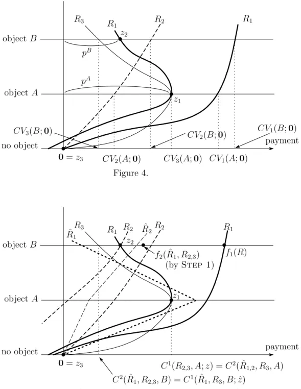
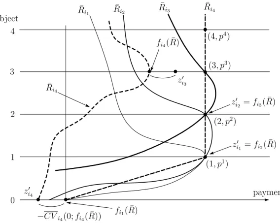
Case V: Nonquasi-linear domain (two-object case, 3). Finally, we consider the case where agents’ preferences are depicted in Figure 4. The compensating valuations from the origin are ranked as CV

(A; 0) > CV

(A; 0) > CV

(A; 0) and CV

(B; 0) > CV

(B; 0) >

CV

(B; 0). In this case, the outcome of the MPW rule is as follows: Agent 1 receives object A and pays CV

(A; 0), i.e., the price p

of object A is CV

(A; 0). This agent 1’s consumption point is depicted as z

in Figure 4. Agent 2 receives object B and pays CV

(B; z

), i.e., the price p

of object B is CV

(B; z

). This agent 2’s consumption point is depicted as z

in Figure 4. In this case, it is agent 1’s preference that decided whether agent 2 or 3 receives an object. In Figure 4, agent 1 prefers (A, CV

(A; 0)) to (B, CV

(B; 0)), and agent 2 receives an object. However, if agent 1 prefers (B, CV

(B; 0)) to (A, CV

(A; 0)), agent 3 instead receives an object.

Similar to above Case IV, it is easy to see why this allocation is the outcome of the MPW rule, and coincides with the outcome of the SA auction. As in Case IV, the price of object B is not any agent’s compensating valuation of object B from the origin, the MPW outcome does not coincide with the VCG rule from 0, and efficient allocation of objects cannot be obtained simply by maximizing the sum of agents’ compensating valuations from the origin.

[Figure 4 about here]

In the above five cases, we contrasted the MPW rule with the VCG rule. Outcomes of the two rules coincide in Cases I, II and III, but not in Cases IV and V. The VCG rule above employs only a small part of the information about agents’ preferences (i.e.,

“compensating valuations from the origin”). On the other hand, the MPW rule employs other information (i.e., “compensating valuations from various points”). As we show in the remainder of this article, only the MPW rule satisfies strategy-proofness, Pareto-efficiency, individual rationality, and nonnegative payment on the domain including nonquasi-linear preferences. Thus, the information about compensating valuations from various points is necessary to design rules satisfying the above four properties on this domain.

As Demange, Gale, and Sotomayor (1986), etc., discuss and we show formally in Sec- tion 6, the outcome of the SA auction always coincides with the minimum price Walrasian equilibrium allocation.

3 The Model and Definitions

There are n agents and m objects, where 2 ≤ n < ∞ and 1 ≤ m < ∞ . We denote the set of agents by N ≡ { 1, . . . , n } , and the set of objects by M ≡ { 1, . . . , m } . Let L ≡ { 0 } ∪ M.

Each agent is permitted to receive one object at most. We denote the object that agent i ∈ N receives by x

∈ L. Object 0 is referred as the “null object”, and x

= 0 means that agent i receives no object. We denote the money that agent i pays by t

∈ R . For each i ∈ N , agent i’s consumption set is L × R , and agent i’s (consumption) bundle is a pair z

≡ (x

, t

) ∈ L × R . Let 0 ≡ (0, 0).

Each agent i has a complete and transitive preference relation R

on L × R . Let P

and I

be the strict and indifference relation associated with R

, respectively. Given a preference R

and a bundle z

∈ L ×R , we denote the upper contour set and lower contour set of R

at z

by the sets U C (R

, z

) ≡ { z ˆ

∈ L × R : ˆ z

R

z

} and LC(R

, z

) ≡ { z ˆ

∈ L × R : z

R

z ˆ

} , respectively. We assume that a preference satisfies the following properties:

Continuity: For each z

∈ L × R , U C(R

, z

) and LC(R

, z

) both are closed.

Money monotonicity: For each x

∈ L and each t

, t ˆ

∈ R , if ˆ t

< t

, then, (x

, ˆ t

) P

(x

, t

).

Finiteness: For each t

∈ R , each x

, x ˆ

∈ L, there is ˆ t

∈ R such that (ˆ x

, t ˆ

) R

(x

, t

).

Let R

be the class of continuous, money monotonic, and finite preferences, which we call the “extended domain”. Given R

∈ R

, z

∈ L × R , and y

∈ L, we define compensating valuation CV

(y

; z

) of y

from z

for R

by (y

, CV

(y

; z

)) I

z

. Note that by continuity and finiteness of preferences, CV

(y

; z

) exists, and by money monotonicity, CV

(y

; z

) is unique. The compensating valuation for ˆ R

is denoted by CV d

.

We introduce another property of preferences.

Desirability of objects: For each x

∈ M and each t

∈ R , (x

, t

) P

(0, t

).

Definition 3.1. A preference R

is classical if it satisfies continuity, money monotonicity, finiteness, and desirability of objects.

12The following is a weaker condition of desirability of objects. A preference R_i satisfies weak desirability of objects if for each x_i∈M, (x_i,0)P_i0. All the results in this article still hold if desirability of objects is replaced by weak desirability.

Let R

be the class of classical preferences, which we call the “classical domain”. Note that R

( R

.

Definition 3.2. A preference R

is quasi-linear if there is a valuation function v

: L → R

such that v

(0) = 0, and for each z

≡ (x

, t

) ∈ L × R , and each ˆ z

≡ (ˆ x

, ˆ t

) ∈ L × R , z

R

z ˆ

⇐⇒ v

(x

) − t

≥ v

(ˆ x

) − ˆ t

.

We denote the class of quasi-linear preferences by R

, which we call the “quasi-linear domain”.

An object allocation is an n-tuple (x

, . . . , x

) ∈ L

such that for each i, j ∈ N , if x

6 = 0 and i 6 = j , then x

6 = x

, that is, any two agents do not receive the same object. Let X be the set of object allocations. A (feasible) allocation is an n-tuple z ≡ (z

, . . . , z

) of bundles such that (x

, . . . , x

) ∈ X. Let Z be the set of feasible allocations. We denote the object allocation and agents’ payments under an allocation ˆ z by ˆ x ≡ (ˆ x

, . . . , x ˆ

) and t ˆ ≡ (ˆ t

, . . . , t ˆ

), respectively.

Let R be a class of preferences such that R ⊆ R

. A preference profile is an n-tuple R ≡ (R

, . . . , R

) ∈ R

. Given R ≡ (R

, . . . , R

) ∈ R

and N

⊆ N , let R

≡ (R

)

and R

≡ (R

)

.

An allocation rule, or simply a rule, on R

is a function f from R

to Z. Given a rule f and a preference profile R ∈ R

, we denote agent i’s assignment of objects under f at R by f

(R) and i’s payment under f at R by f

(R), and we write

f

(R) ≡ (f

(R), f

(R)), f (R) ≡ (f

(R), . . . , f

(R)), and f

(R) ≡ f

(R)

. We introduce basic properties of rules. The efficiency condition defined below takes the auctioneer’s preference into account and assumes that he is indifferent to the auctioned objects, that is, he is only interested in his revenue. An allocation z ∈ Z is Pareto-efficient for R ∈ R

if there is no feasible allocation ˆ z ∈ Z such that

(i) X

i∈N

ˆ t

≥ X

i∈N

t

, (ii) for each i ∈ N, z ˆ

R

z

, and (iii) for some j ∈ N, z ˆ

P

z

. For each R ∈ R

, let P (R) be the set of Pareto-efficient allocations for R.

Efficiency: For each R ∈ R

, f (R) ∈ P (R).

Individual rationality defined below requires that a rule should never assign an alloca- tion which makes some agent worse off than he would be if he had received no object and paid nothing. Nonnegative payment requires that the payment of agents always should be nonnegative.

Individual rationality: For each R ∈ R

and each i ∈ N , f

(R) R

0.

Nonnegative payment: For each R ∈ R

and each i ∈ N , f

(R) ≥ 0.

The two properties below are of incentive-compatibility. The first says that by misrepre- senting his preferences, no agent should obtain an assignment that he prefers.

Strategy-proofness: For each R ∈ R

, each i ∈ N , and each ˆ R

∈ R , f

(R) R

f

( ˆ R

, R

).

The second is a stronger property: by misrepresenting their preferences, no group of agents should obtain assignments that they prefer.

Group strategy-proofness: For each R ∈ R

and each ˆ N ⊆ N , there is no ˆ R

∈ R

such that for each i ∈ N ˆ , f

( ˆ R

, R

) P

f

(R).

4 Minimum Price Walrasian Equilibrium

We define “Walrasian equilibrium” and “minimum price Walrasian equilibrium” in this model. As Demange, Gale, and Sotomayor (1986), etc., explain, and we show in Section 6, the minimum price Walrasian equilibria coincide with the outcomes of SA auctions. Let R ⊆ R

in this section. All results in this section also hold on the classical domain R

.

Given a price vector p ≡ (p

, . . . , p

) ∈ R

of m objects, the budget set (or available set) is defined as B(p) ≡ { (x, p

) : x ∈ L } , where p

= 0 if x = 0. Given R

∈ R and p ∈ R

, agent i’s demand set D(R

, p) is defined as D(R

, p) ≡ { x ∈ L : ∀ y ∈ L, (x, p

) R

(y, p

) } .

Next is the definition of “Walrasian equilibrium”.

Definition 4.1. Let R ∈ R

. A pair (z, p) ∈ Z × R

of feasible allocation and price vector is a Walrasian equilibrium for R if it satisfies the following two conditions:

(WE-i) for each i ∈ N , x

∈ D(R

, p) and t

= p

,

(WE-ii) for each x ∈ M, if for each i ∈ N, x

6 = x, then, p

= 0.

Condition (WE-i) says that each agent receives the object he demands, and pays its price.

Condition (WE-ii) says that an object’s price is zero if it is not assigned.

Fact 4.1. For each R ∈ R

, there is a Walrasian equilibrium for R.

Fact 4.1 is already proven in the literature. For example, see Alkan and Gale (1990).

Our model is a special case of their model. In Section 6, we give an alternative proof of the existence of Walrasian equilibrium as Proposition 6.1 by using the SA auction.

Given R ∈ R

, let W (R) be the set of Walrasian equilibrium allocations for R, that is, z ∈ W (R) if and only if there is a price vector p ∈ R

such that the pair (z, p) is a Walrasian equilibrium for R. Fact 4.2 below is so-called First Welfare Theorem.

Fact 4.2. Let R ∈ R

and z ∈ W (R). Then, z is Pareto-efficient for R.

Fact 4.3 below says that for each preference profile, there is a minimum price Walrasian equilibrium.

13Let #Adenote the cardinality of setA.

14To see this, suppose that z ≡(z₁, . . . , z_n) is notPareto-efficient for R. Then, there is ˆz ≡(ˆz₁, . . . ,zˆ_n) such that

(i) X

i∈N

ˆtⁱ≥X

i∈N

tⁱ, (ii) for each i∈N,zˆiRizi, (iii) for somej∈N,zˆjPjzj.

Since z ∈W(R), there is a price vectorp∈R^m+ such that (z, p) is a Walrasian equilibrium forR. Then, by (ii) and (WE-i), for each i∈N, ˆt_i ≤p^ˆxi. By (iii) and (WE-i), ˆt_j < p^xˆj. Thus, P

i∈Nˆt_i <P

i∈Np^xˆi = P

i∈Nt_i. This contradicts (i).

Fact 4.3 (Demange and Gale, 1985). Let R ∈ R

. There is a Walrasian equilibrium (z

, p

) ∈ Z × R

for R such that, for each price vector p ∈ R

, if there is z ∈ Z such that the pair (z, p) is a Walrasian equilibrium for R, then for each x ∈ M , p

≤ p

.

Given R ∈ R

, let W

(R) be the set of the minimum price Walrasian equilibrium allocations for R. That is, z ∈ W

(R) if and only if there is p

∈ R

such that the pair (z, p

) is a minimum price Walrasian equilibrium for R. By Facts 4.1 and 4.3, for each R ∈ R

, the set W

(R) is nonempty. Although the correspondence W

is set valued, but it is essentially single-valued. That is, for each R ∈ R

, each pair z, z

∈ W

(R), and each i ∈ N , z

I

z

.

We denote the minimum Walrasian equilibrium price for R by p

(R).

Next, we introduce the concepts of “overdemanded set” and “underdemanded set” (De- mange, Gale, and Sotomayor, 1986; Mishra and Talman, 2010). We relate these concepts to Walrasian equilibria.

Definition 4.2. A set M

⊆ M of objects is (weakly) overdemanded at p for R if

# { i ∈ N : D(R

, p) ⊆ M

} ( ≥ ) > #M

. A set M

⊆ M of objects is (weakly) underdemanded at p for R if

[ ∀ x ∈ M

, p

> 0] = ⇒ # { i ∈ N : D(R

, p) ∩ M

6 = ∅} ( ≤ ) < #M

.

Fact 4.4 below is shown by Mishra and Talman (2010) under the assumption that prefer- ences are quasi-linear. However, their proof does not depend on this assumption.

Fact 4.4 (Mishra and Talman, 2010). Let R ∈ R

. A price vector p is a Walrasian equilibrium price for R if and only if no set of objects is overdemanded and no set of objects is underdemanded at p for R.

Theorem 4.1 below is a characterization of the minimum price Walrasian equilibrium by means of the concepts of overdemanded and weakly underdemanded sets. Mishra and Talman (2010) first obtain the same conclusion on the quasi-linear domain. We emphasize, in contrast to Fact 4.4, that Mishra and Talman’s (2010) proof crucially depends on the quasi-linearity. It relies on a simple fact that when preferences are quasi-linear, if a set M

of objects is weakly underdemanded at a Walrasian equilibrium (z, p), then all the prices of M

can be slightly lowered by the same amount while maintaining the Walrasian equilibrium conditions (WE-i) and (WE-ii). However, it is not true when preferences are not quasi-linear.

Theorem 4.1 below is a novel result in that point.

Theorem 4.1 is the key to obtaining all the important results introduced in the subsequent sections, such as Theorem 5.1 in Section 5 and Proposition 6.1 in Section 6. As mentioned earlier, we obtain the existence of Walrasian equilibrium as a byproduct of Proposition 6.1.

Thus, this theorem is also a key to the existence of Walrasian equilibrium.

Theorem 4.1. Let R ∈ R

. A price vector p is a minimum Walrasian equilibrium price for R if and only if no set of objects is overdemanded and no set of objects is weakly underdemanded at p for R.

15They also show that for each preference profile, there is a maximum price Walrasian equilibrium.

16An allocation z⁰ ∈Z is obtained by an indifferent permutation from z ∈ Z if there is a permutationπ onN such that for alli∈N,z_i⁰=z_π(i)andz_i⁰I_iz_i (Tadenuma and Thomson, 1991). Note that for each pair z, z⁰ ∈W_min(R),z⁰ is obtained by an indifferent permutation from z.

The following structures of the minimum price Walrasian equilibrium are obtained as a corollary of Theorem 4.1. Corollary 4.1 says that if the number of objects is greater than or equal to the number of agents, the price of some objects is 0. Corollary 4.2 says that each object bearing a positive price is connected by agents’ demands to the null object or to an object with a price of 0.

Corollary 4.1 (Existence of Free Object). Let m ≥ n, R ∈ R

, and z ∈ W

(R).

Then, there is i ∈ N such that p

(R) = 0.

Corollary 4.2 (Demand Connectedness).

Let R ∈ R

and (z, p) be a minimum Wal- rasian equilibrium price for R. For each x ∈ M with p

> 0, there is a sequence { i

}

of K distinct agents such that (i) x

= 0 or p

= 0, (ii) x

= x, and (iii) for each k ∈ { 1, . . . , K − 1 } , { x

, x

} ⊆ D(R

, p).

Proofs of Theorem 4.1 and Corollaries 4.1 and 4.2 appear in the Appendix.

5 Main Results

In this section, we provide a characterization of the minimum price Walrasian equilibrium by means of the properties of rules.

Let R ⊆ R

. Let g be a rule such that for each R ∈ R

, g(R) ∈ W

(R). Then, g is called a selection from the minimum price Walrasian equilibrium, which we call a minimum price Walrasian rule.

5.1 Properties of the Minimum Price Walrasian Rule

We discuss the properties of the minimum price Walrasian rule. Let g be a minimum price Walrasian rule on R

. First, by Fact 4.2, for each R ∈ R

, g(R) is Pareto-efficient for R. Let R ∈ R

. Then, there is a price vector p ≡ (p

, . . . , p

) ∈ R

such that for each i ∈ N , (a) g

(R) ∈ B(p), and (b) for each ˆ z

∈ B(p), g

(R) R

z ˆ

. Let i ∈ N . Note that, for each x ∈ M, p

≥ 0, and B(p) = { (0, 0), (1, p

), (2, p

), . . . , (m, p

) } . Thus, by (a), g

(R) ≥ 0, and by (b), g

(R) R

0. Therefore, the minimum price Walrasian rules satisfy efficiency, individual rationality, and nonnegative payment.

Fact 5.1 below was first shown by Demange and Gale (1985). By using Theorem 4.1 in Section 4, we show this fact more directly in the Appendix.

Fact 5.1 (Demange and Gale, 1985). The minimum price Walrasian rules are group strategy-proof.

5.2 Characterizations

In this subsection, we focus on the analysis in the case where each agent has a classical preference and the number of agents exceeds the number objects. Remember that all results established in Section 4 also hold in this case. Theorem 5.1 below is a main conclusion of this article, a characterization of the minimum price Walrasian rule.

Theorem 5.1. Let R ≡ R

and n > m. A rule f on R

satisfies strategy-proofness, efficiency, individual rationality, and nonnegative payment if and only if it is a minimum price Walrasian rule: for each R ∈ R

, f(R) ∈ W

(R).

17This structure is discussed by Demange, Gale, and Sotomayor (1986) and Miyake (1998).

Since the minimum price Walrasian rules are group strategy-proof, we obtain the following as a corollary of Theorem 5.1.

Corollary 5.1. Let R ≡ R

and n > m. A rule f on R

satisfies group strategy-proofness, efficiency, individual rationality, and nonnegative payment if and only if it is a minimum price Walrasian rule.

Proof of Theorem 5.1 is in the Appendix. In addition, we give an overview of the proof in Section 7.

5.3 Independence of the Axioms

The only if part of Theorem 5.1 fails if we drop any of the four axioms. The following examples establish the independence of the axioms in Theorem 5.1.

Example 1 (Dropping strategy-proofness ). Let f be a rule that chooses a “maximum”

price Walrasian equilibrium allocation for each preference profile. Then, the rule f satisfies efficiency, individual rationality, and nonnegative payment, but not strategy-proofness.

Example 2 (Dropping efficiency ). Let f be the rule such that for each preference profile, each agent receives no object and pays nothing. Then, the rule f satisfies strategy-proofness, individual rationality, and nonnegative payment, but not efficiency.

Next, we introduce variants of Walrasian equilibrium, one with “entry fee”. Let R ∈ R

and t

∈ R . A pair (z, p) ∈ Z × R

of feasible allocation and price vector is a Walrasian equilibrium with “entry fee t

” for R if (i) p

= t

and for each x ∈ M , p

≥ t

, (ii) for each i ∈ N and each y ∈ L, (x

, p

) R

(y, p

) and t

= p

, and (iii) for each x ∈ M , if for each i ∈ N , x

6 = x, then p

= t

. Note that, by Facts 4.1 and 4.3, for each preference profile and each entry fee t

, there is a minimum price Walrasian equilibrium with entry fee t

. Moreover, we remark that, by Fact 5.1, for each entry fee t

, any selection from the minimum price Walrasian equilibrium with entry fee t

is (group) strategy-proof.

Example 3 (Dropping individual rationality ). Let t

> 0. Let f be a rule that chooses a minimum price Walrasian equilibrium with positive entry fee t

for each preference profile.

Then, the rule f satisfies strategy-proofness, efficiency, and nonnegative payment, but not individual rationality.

Example 4 (Dropping nonnegative payment ). Let t

< 0. Let f be a rule that chooses a minimum price Walrasian equilibrium with negative entry fee t

for each preference profile.

Then, the rule f satisfies strategy-proofness, efficiency, and individual rationality, but not nonnegative payment.

6 Simultaneous Ascending Auction

In this section, we define a class of simultaneous ascending auctions, and show that they achieve the minimum price Walrasian equilibrium. Let R ⊆ R

.

Definition 6.1. Given R ∈ R

and p ∈ R

, a set M

⊆ M of objects is a minimal

overdemanded set at p for R if M

is overdemanded at p for R, and there is no M

( M

such that M

is overdemanded at p.

Under a (continuous time) “simultaneous ascending auction”, in each time, each bidder submits his demand at a current price vector, and the prices of the objects in a minimal overdemanded set are raised at a speed at least d > 0.

Definition 6.2. A simultaneous ascending (SA) auction is a function ˆ p from R

× R

× R

to R

such that

(i) for each p ∈ R

, each R ∈ R

, and each x ∈ M , ˆ p

(0, p, R) ≡ 0,

(ii) there is d > 0 such that for each t ∈ R

, each p ∈ R

, each R ∈ R

, and each x ∈ M , (ii-a) dˆ p

(t, p, R)/dt ≥ d if x is in a minimal overdemanded set at p for R, and

(ii-b) dˆ p

(t, p, R)/dt = 0 otherwise.

Remark 6.1. For each R ∈ R

, an SA auction ˆ p generates a price path p( · ) such that for each x ∈ M and each t ∈ R

,

p

(t) = Z

0

dˆ p

(s, p(s), R) ds ds.

Proposition 6.1. For each preference profile, the price path generated by any simultaneous ascending auction converges to the minimum Walrasian equilibrium price in a finite time.

The proof is in the Appendix. Proposition 6.1 says that for each R ∈ R

, the price path p( · ) generated by an SA auction has a final time T such that for each t ≥ T , p(t) = p(T ) = p

(R), and at the final price p(T ), each agent receives an object from his demand.

Moreover, this proposition shows the existence of Walrasian equilibrium.

7 Overview of the proof of Theorem 5.1

We give an overview of the proof of Theorem 5.1. Since if part of the theorem follows from the discussion in Subsection 5.1, we explain the proof of only if part of the theorem.

As we emphasized in Introduction, without quasi-linearity of preferences, efficient alloca- tions of objects depend on payments. Thus, it is difficult to identify the object allocations of the rules satisfying our desirable properties without knowing their payments. On the other hand, it is also difficult to identify the payments of the rules satisfying our properties with- out knowing their object allocations. In this section, we discuss how we overcome those dual difficulties.

Let R ≡ R

and n > m. The proof consists of the following four parts.

PART 1. We show the four preliminary results below, which are repeatedly used in the proof.

Lemma 5.1 below says that under individual rationality and nonnegative payment, when- ever an agent does not receive any object, then the payment of the agent should be zero.

Lemma 5.1. Let f be a rule that satisfies individual rationality and nonnegative payment on R

. Let R ∈ R

and i ∈ N be such that f

(R) = 0. Then, f

(R) = 0.

Lemma 5.2 says that under efficiency, individual rationality, and nonnegative payment,

each object should be assigned to someone.