INVITED SURVEY PAPER
Radio Techniques Incorporating Sparse Modeling
Toshihiko NISHIMURA†a),Senior Member, Yasutaka OGAWA†, Takeo OHGANE†,Fellows, andJunichiro HAGIWARA†,Member
SUMMARY Sparse modeling is one of the most active research areas in engineering and science. The technique provides solutions from far fewer samples exploiting sparsity, that is, the majority of the data are zero. This paper reviews sparse modeling in radio techniques. The first half of this pa- per introduces direction-of-arrival (DOA) estimation from signals received by multiple antennas. The estimation is carried out using compressed sens- ing, an effective tool for the sparse modeling, which produces solutions to an underdetermined linear system with a sparse regularization term. The DOA estimation performance is compared among three compressed sensing algorithms. The second half reviews channel state information (CSI) acqui- sitions in multiple-input multiple-output (MIMO) systems. In time-varying environments, CSI estimated with pilot symbols may be outdated at the actual transmission time. We describe CSI prediction based on sparse DOA estimation, and show excellent precoding performance when using the CSI prediction. The other topic in the second half is sparse Bayesian learning (SBL)-based channel estimation. A base station (BS) has many antennas in a massive MIMO system. A major obstacle for using the massive MIMO system in frequency-division duplex mode is an overhead for downlink CSI acquisition because we need to send many pilot symbols from the BS and to get the feedback from user equipment. An SBL-based channel estimation method can mitigate this issue. In this paper, we describe the outline of the method, and show that the technique can reduce the downlink pilot symbols.
key words: sparse modeling, compressed sensing, sparse Bayesian learn- ing, DOA estimation, channel estimation
1. Introduction
Radio techniques have developed rapidly for these decades.
Especially, mobile communication has evolved almost every ten years. Many technologies supporting the fifth generation (5G) have been extensively studied [1]–[6], and commer- cial 5G services are being deployed in several countries.
More recently, the evolution beyond 5G or toward 6G is be- ing discussed[7],[8]. Various signal processing techniques enable advanced wireless communication. One of them is a multiple-input multiple-output (MIMO) system, in which both of the transmitter and the receiver have multiple anten- nas[9],[10]. The MIMO technique, space-domain signal processing, makes it possible to realize high-speed trans- mission using space division multiplexing[11]. Other than mobile communication, radio technologies have been widely studied in several fields such as radars and wireless sensor networks[12]–[16].
Manuscript received May 29, 2020.
Manuscript revised August 4, 2020.
Manuscript publicized September 1, 2020.
†The authors are with the Faculty of Information Science and Technology, Hokkaido University, Sapporo-shi, 060-0814 Japan.
a) E-mail: [email protected] DOI: 10.1587/transfun.2020EAI0001
On the other hand, sparse modeling has been collect- ing considerable attention in several fields. The signal pro- cessing technique is a framework which provides solutions exploiting sparsity, that is, the majority of the data are equal to zero. Several important concepts are discussed in[17].
Compressed sensing or compressive sensing is an effective tool for the sparse modeling[18]–[30]. One of the biggest successes of the method is magnetic resonance imaging (MRI), which has been widely used for medical diagnosis due to its high resolution and noninvasive merits[31],[32].
Another breathtaking result is black hole imaging achieved by the Event Horizon Telescope Collaboration[33]–[39].
Compressed sensing plays a crucial role also in radio techniques. We need channel state information (CSI) for wireless communication. CSI is essential for detection at a receiver, and is also required for MIMO precoding at a trans- mitter. In radio engineering, information is transmitted by radio waves. The waves are inevitably affected by propaga- tion environments, that is, they are reflected, scattered, and diffracted from the surrounding objects, and are received as multipath signals. These multipath signals determine channels. According to channel measurement campaigns [40], [41], multipath components do not arrive uniformly from all angles of arrival but as clusters. This propagation property holds also in the delay domain, and we can assume that wireless channels are sparse in spatial and temporal do- mains. Thus, many researches have been done for channel estimation with compressed sensing such as[42]–[50].
Another research area is high-resolution direction-of- arrival (DOA) estimation of radio waves, which is of great importance in such as radar, position estimation, radio as- tronomy, and CSI estimation in MIMO systems. The re- search dates back to the 1960s[51], and has been continued until today[52]–[55]. In sparse radio environments, DOA estimation based on compressed sensing has significant ben- efits such as smaller number of snapshots required and has ability to deal with coherent signals, therefore many refer- ences have been published for example[56]–[61]. Further- more, the DOA estimation technique that uses compressed sensing and a generalized MUSIC criterion has been pro- posed[62]. The method can reduce the number of antenna elements.
Based on these research backgrounds, we review sparse modeling in radio techniques. The first half of this paper in- troduces DOA estimation using compressed sensing. After taking a quick look at sparse modeling and formulating the Copyright © 2021 The Institute of Electronics, Information and Communication Engineers
problem as array signal processing, we will explain sparse DOA estimation algorithms. The second half reviews MIMO CSI acquisition methods. In time-varying environments, CSI estimated with pilot symbols may be outdated at the actual transmission time. One of the solutions to this issue is channel prediction based on sparse DOA estimation[63], which can provide a long prediction range. We describe the technique in detail. The other topic to be introduced in the second half is sparse Bayesian learning (SBL)-based channel estimation. A base station (BS) has many antennas in a mas- sive MIMO system[64],[65]. A major obstacle for using the massive MIMO system in frequency-division duplex (FDD) mode is an overhead for downlink CSI acquisition, that is, we need to send many pilot symbols from the BS and to get the feedback from user equipment (UE)[66]–[68]. Dai et al.[69]have proposed an SBL-based channel estimation method to mitigate this issue, which will be discussed later.
Introduction of the above two channel acquisition methods will be beneficial to readers who are interested in sparse modeling in radio techniques.
The rest of the paper is organized as follows. In Sect. 2, we briefly review sparse modeling and compressed sensing.
In Sect. 3, we explain the basics of array signal process- ing and DOA estimation based on compressed sensing. In Sect. 4, we introduce channel prediction using the DOA es- timation in time-varying environments and downlink SBL- based channel estimation in an FDD massive MIMO system.
Conclusions follow in Sect. 5.
2. Brief Review of Sparse Modeling and Compressed Sensing
This section briefly describes sparse modeling and com- pressed sensing algorithms used for DOA estimation in Sects. 3 and 4. For interested readers, refer to review pa- pers or books such as[27],[28],[70],[71],[73]for further details on this research area.
We consider the following simultaneous linear equa- tions
y=Ax, (1)
where y and x are M-dimensional and N-dimensional complex-valued vectors, respectively, and A is an M×N complex-valued matrix. We want to solve the unknown vec- torx for giveny andA. We assume M < N, that is, the number of equations is less than that of unknowns. In this case, (1) is called underdetermined systems, and its solution is not unique. Infinitely many vectorsxsatisfy (1).
Here, we assume that x is sparse, that is, most of the elements are zero. Due to the sparsity, it is natural to obtain the solution x that has the least non-zero elements. We define a vector 0-norm (`0-norm) as the number of non-zero elements inx, and denote it askxk0. Then, the solution is given by
minx kxk0 subject to y=Ax. (2)
Unfortunately, the 0-norm minimization is unrealistic be- cause of the expected combinatorial explosion as the dimen- sion ofxincreases.
We introduce a vectorp-norm (`p-norm) defined by
kxkp =* ,
XN
i=1
|xi|p+ -
1 p
(p>0). (3)
We replace kxk0 in (2) with kxkp. Furthermore, using a Lagrange multiplierα, we have the following unconstrained minimization
arg min
x
1
2 kAx−yk22+αkxkpp
!
, (4)
The above equation can also treat a case where yincludes noise as stated in later sections. When p ≥ 1, the objec- tive function of (4) is a convex function of the variable x, which allows us to efficiently find an approximate solution by numerical computations. However, it is difficult to obtain a sparse solution with 2-norm (`2-norm) minimization. By using 1-norm (`1-norm) minimization, the sparse solution can be obtained with realistic computational complexities, and many methods have been presented so far [27]. As will be mentioned later, some algorithm uses the value of 0<p<1.
One of the most typical algorithms for the 1-norm min- imization is the fast iterative shrinkage thresholding algo- rithm (FISTA) [74]which is an accelerated version of the iterative shrinkage thresholding algorithm (ISTA), a kind of proximity gradient method. The solution of ISTA is given by the following iteration
x[k+1]=Sα
L
x[k]+L−1AH y−Ax[k]
, (5)
where H denotes Hermitian transpose and Sa(b) is a shrinkage-thresholding function, also known as a soft thresh- old function, defined by
Sa(b)=
( |b|−a
|b|
b (a <|b|)
0 (otherwise) . (6)
Note that the function is applied to each element of the vector.
Furthermore,Lis a parameter satisfying
L≥ kAHAk. (7)
Here, kAHAk denotes the maximum eigenvalue of AHA, which is the Lipschitz constant of the gradient of(1/2)kAx− yk2
2. Note that when x,y, and Aare real-valued, the Her- mitian transpose in the above expressions is replaced with transpose[27].
In FISTA, to accelerate the convergence, we slightly change the iteration as follows
x[0] :=AHy.
w[1] :=x[0].
β:=1.
k:=1.
loop
x[k] :=Sα/L(w[k]+L−1AH y−Aw[k]. β[k+1] :=12 +q
1
4 +β[k]2.
w[k+1] :=x[k]+β[kβ[k]−1+1](x[k]−x[k−1]). k:=k+1.
end loop
It is seen that Aw[k] requires M N complex multipli- cations. Since AH and(y−Aw[k])are an N×M matrix and anM-dimensional vector, respectively, the matrix-vector multiplication AH(y−Aw[k])needs N Mcomplex multi- plications. Thus, the computational complexity at each step isO(M N).
Now, we consider the half-quadratic regularization (HQR) method [76]. In HQR, p < 1 is usually used in (4). The algorithm is formulated deleting the constant 1/2 in (4) in [76]. In order to avoid problems due to non- differentiability of the `p-norm around the origin when p ≤ 1, the following smooth approximation is applied to (3).
kxkp≈* ,
N
X
i=1
(|xi|2+)p/2+ -
1/p
. (8)
Here, ≥0 is a small constant. HQR obtains the solution by the iteration
x[k+1]=H(x[k])−1AHy, (9)
where
H(x)=AHA+αΛ(x) (10)
Λ(x)=diag
p 2
(|xi|2+)1−p2
. (11)
In (11), diag{·}denotes a diagonal matrix whoseith diagonal element is the expression inside the brackets.
It is seen that we can calculateAHyand AHAin ad- vance before the iteration. SinceH(x)is anN×Nmatrix, we need complex multiplications in the order ofN3to carry out the inversionH(x[k])−1in (9). Furthermore,AHyis an N-dimensional vector, and the matrix-vector multiplication H(x[k])−1AHyrequiresN2complex multiplications. Con- sequently, we needO(N3)complex multiplications at each step. The computational load is heavy because N usually has a large value.
Finally, we introduce the Orthogonal Matching Pursuit (OMP), which is one of the greedy algorithms [22],[23].
OMP is not based on (4) but obtains the support set of x denoted byΩ. We express theK-dimensional vector whose elements consist of x in Ω as xΩ, where K denotes the number of non-zero elements in x. We also represent the matrix deleting the columns exceptΩfromAasAΩ, which is anM×Kmatrix. UsingxΩandAΩ, (1) is rewritten as
y=AΩxΩ. (12)
From the sparsity ofx,K <Mholds, and we can solve (12) forxΩ. The solution is given as
xΩ= AΩHAΩ
−1
AHΩy. (13)
We iteratively obtain the support setΩ. LetΩ[k] andr[k]
denote the kth support set and residualy−AΩ[k]xΩ[k], re- spectively. We start with Ω[0] = φ and xΩ[0] = 0, i.e., r[0]=y. Moreover, we express the jth column ofAas aj. At each iteration, we findaj most correlated with the resid- ual, and include the column number into the support. Based on this concept, we update the support set in the following manner[27],[71].
Ω[0] :=φ.
xΩ[0]:=0.i.e.,r[0]=y−AxΩ[0]=y.
k:=0.
loop
J[k+1] :=arg maxj |a
H jr[k]|
kajk2 . Ω[k+1] :=Ω[k]∪ {J[k+1]}.
xΩ[k+1]:=
AΩ[k+1]H AΩ[k+1]−1
AΩ[k+1]H y.
r[k+1] :=y−AΩ[k+1]xΩ[k+1]. k:=k+1.
end loop
Sinceajandr[k] areM-dimensional vectors, we need M complex multiplications to calculate the scalar prod- uct aHj r[k]. In the kth loop of the iteration, we need M(N−k)complex multiplications to obtainaj that maxi- mizes|aHj r[k]|/kajk2. Note that(k−1)vectors have been chosen up to the(k−1)th loop, and we only need to search for the vectorajamong the remaining(N−k)ones. Further- more,xΩ[k+1]andr[k+1] requirek(k M+M+k)+O(k3) and k M complex multiplications for their updates, respec- tively. In total, we need O(max(M N,k2M,k3)) complex multiplications in thekth loop.
We have considered computational complexities at each step of the algorithms. It would depend on an algorithm how many steps we need for convergence. The authors advise interested readers to try simulations.
3. DOA Estimation of Electromagnetic Waves
Estimating DOAs of radio waves from signals received by multiple antennas is a typical example of array signal pro- cessing. The handling of signals linearly observed by an array antenna can be described by simultaneous linear equa- tions. We usually need to treat an underdetermined linear system with less observation data than the number of un- knowns (original signals). However, when the original sig- nal is sparse, the exact solution can be obtained by a concept called compressed sensing. In this section, we introduce DOA estimation with compressed sensing and compare the performance of three algorithms.
3.1 Basics of DOA Estimation with Array Antenna Figure 1 is a diagram of a DOA estimation system using an
Fig. 1 DOA estimation with array antenna.
array antenna for a single source case. It is assumed that the source is so far away that the radio wave is incident as a plane wave on the array antenna, and the radio wave experiences phase rotation between antenna elements according to the path difference shown in Fig. 1. Therefore, the DOA of the radio wave can be estimated by calculating the path differ- ence between the elements from the phase difference. As can be seen from Fig. 1, to calculate the DOA of a single wave, the array antenna needs only two elements. If the positions of the two antenna elements are known exactly, the DOA can be readily calculated. However, the received signal contains noise in addition to errors such as IQ imbalance due to the fabrication process of the device. Although the latter can be offset or mitigated by calibration, it is impossible to com- pletely remove the effects of noise, and the estimated DOA inevitably has an error. Furthermore, in general, we have plural sources and multipaths. DOA estimation has been a challenging issue for radio researchers, and has a long re- search history [72]. In the next subsection, we introduce compressed sensing-based DOA estimation.
3.2 Application of Compressed Sensing
As shown in Fig. 2, we assume that K narrowband signals are incident on a uniform linear array (ULA) of M omni- directional elements. Also, as seen from Fig. 2, we divide the angular domain into N small regions, each of which is called a “bin”. We definexn(t)as a signal arriving from the direction of thenth bin at timet. If no signal arrives from it, xn(t) =0 holds. We express an N-dimensional column vector consisting of xn(t)as x(t), which is called an orig- inal signal vector. For example, when signals are incident from the directions of the third andnth bins, the original sig- nal vector is x(t) = [0, 0, x3(t), 0, . . .0, xn(t), 0, . . .0]T, where [ ]Tdenotes transpose. We see that the DOAs of ar- riving signals can be estimated from the support ofx(t).
Next, we introduce anM×Nmatrix Awhose the (m, n)th element is given by
amn=ej2πλdmsinθn, (14) whereλ,dm, and θn are the wavelength corresponding to
Fig. 2 DOA estimation model for compressed sensing.
the frequency of the arriving wave, the distance of themth antenna element from a reference point, and the angle of the center of the nth bin, respectively. We refer to the center of each bin as a grid point. Each column vector of A is a steering vector for the angle θn. Note that Ais called a steering matrix, an observation matrix, or a sensing matrix.
We denote anM-dimensional column vector whosemth element is a received signal at themth antenna at timet as y(t). The vector is given by
y(t)=Ax(t)+n(t), (15) where n(t) is an M-dimensional noise vector. Note that throughout this paper, we assume additive Gaussian noise that is independent spatially and temporally.
In (15),y(t),x(t), andn(t)are continuous-time waves.
We assume that the DOAs of arriving signals do not change during a limited time period. Sampling (15), we can estimate x(t). Moreover, if the complex envelopes of x(t) do not change temporally during the period, we can improve SNR averaging plural snapshot measured data. We assume that the number of arriving signals K is much less than that of bins N, so x(t) is a sparse vector. Thus, the Eq. (15) becomes an underdetermined system with a sparse solution.
The relationship among the number of arriving signals K and the dimensionsx(t)andy(t)is given by
K<M <N. (16)
From the above, it is seen that we can obtain x(t) using compressed sensing stated in Sect. 2, and we can estimate the DOAs of arrival signals.
3.3 Example of DOA Estimation Using Compressed Sens- ing Algorithms
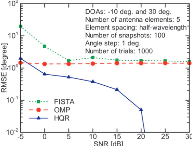
In this subsection, we show an example of DOA estima- tion using FISTA, HQR, and OMP explained in Sect. 2.
The width of each bin shown in Fig. 2 is 1◦, and the grid points are located at integer multiples of 1◦ such as . . . ,−1◦,0◦,1◦,2◦. . .. Two uncorrelated narrow-band waves with the same power impinge on a five-element ULA with half-wavelength spacing. The DOAs are−10◦and 30◦ that coincide with grid points. We assumed that we knew in advance the number of arrival signals 2. We applied each algorithm with a certain convergence condition, and found
Fig. 3 Comparison among three algorithms.
two largest elements in the estimated vector x(t). We con- sidered them as the incident waves, and estimated the DOAs from the supports of them.
Figure 3 shows the root mean square error (RMSE) of the DOA estimation versus SNR. Here, RMSE is defined by
RMSE= vu t1
2I
2
X
k=1 I
X
i=1
θˆk,i−θk
2, (17)
where I is the number of trials, which was 1000 in the simulation. ˆθk,i andθkare the estimated incident angle and the true one of thekth incident wave (k=1,2), respectively.
Here, SNR denotes the signal-to-noise power ratio of each incident wave. From the figure, it can be seen that HQR shows the best estimation result in almost the whole region of the SNR. The reason for this may be due to the value of 0 <p <1. The effects of parameters includingpto the DOA estimation accuracy are discussed in[77]. RMSE in the region of SNR larger than 20 dB was 0. The estimated DOAs coincided with grid points of −10◦ and 30◦, and we had no estimation error in the 1000 trials. As stated previously, however, HQR needs an inversion ofN×Nmatrix every step, and the computational load is heavy. On the other hand, the performance of FISTA was significantly poor at low SNR.
OMP had an error of about 1.5◦, regardless of the SNR. It is interesting that although the computational complexity of OMP is very low, the DOA estimation performance is much better than that of FISTA at the low SNR region. The authors advise readers to carefully consider algorithms before they apply the compressed sensing to their issue.
4. MIMO CSI Acquisition Using Sparse Modeling In this section, we introduce two examples of MIMO CSI acquisition techniques based on DOA estimation. The first is multi-user CSI prediction using compressed sensing in time- varying environments. The second is SBL-based downlink CSI estimation in an FDD massive MIMO system.
4.1 Multi-User MIMO CSI Prediction
Here, we review the basic concept of MIMO CSI predic- tion using two-step compressed sensing[63]. In multi-user MIMO downlink transmission, precoding is done at a BS to prevent inter-user interference and to enhance transmission rates. Downlink CSI is required at the BS for the precod- ing, and is obtained using pilot symbols. In time-varying environments, however, the MIMO channels change during the time interval between channel estimation and actual sig- nal transmission. This causes interference and deteriorates communication quality. If we accurately predict channels from past CSI, we can mitigate the problem. Many pre- diction techniques have been presented so far[78]. Among them, the sum-of-sinusoids (SOS) method predicts channels by resolving an arrival signal to a UE into individual mul- tipath components and summing the predicted ones. If the Doppler frequency and complex amplitude of each multipath component are estimated accurately, we can predict reliable channels for a long prediction range. The SOS method stated below is thus promising. Note that we assume a narrowband system in which we can ignore the delay between multipath components. The considerations below, however, also hold for each subcarrier of OFDM in a broadband system.
A time-varying channel h(t)at a reference point of a UE array from a certain BS antenna is given by
h(t)= XK
k=1
Akej(2πfkt+φk), (18) whereKdenotes the number of multipath components. Also, Ak,φk, and fk denote the amplitude, phase, and Doppler frequency for the kth multipath component, respectively.
From (18), if we obtain the complex amplitudes Akejφkand the Doppler frequencies fk at timet =0 for the multipath components, we can predict future channels for the UE by summing the predicted multipath components.
We resolve the signal into multipath components by es- timating the DOAs. Because the DOAs change relatively slowly, we can assume that they are constant for the channel prediction period. Moreover, we assume that UEs have a uniform circular array (UCA) with M omnidirectional an- tennas, and that the UEs move at a constant speed.
Here, we state the formulation for one UE. For the other UEs, the formulation is the same. We divide the an- gular domain surrounding the UE intoNbins. We represent the observation vectory(t), original signal vectorx(t), and thermal noise vectorn(t)as
y(t) = [y1(t), y2,(t). . . , yM(t)]T (19) x(t) = [x1(t),x2(t), . . . , xN(t)]T (20) n(t) = [n1(t),n2(t), . . . , nM(t)]T. (21) Note that each element inx(t)is a complex amplitude of an incident multipath component. Then, obtaining the original signal vectorx(t)corresponds to DOA estimation as stated in
Sect. 3. The observation vectory(t)consists of the received signal at each UE antenna, and is given by
y(t)=Ax(t)+n(t), (22) whereAis theM×Nobservation matrix.
We use a channel prediction method for a higher fre- quency band such as 20 GHz, where we can consider that the number of multipath componentsK is much fewer thanN [79]. Thus, the original signal vectorx(t)is sparse, and we can apply the compressed sensing technique to obtainx(t).
The HQR method is used for the DOA estimation. This is the first-step compressed sensing.
In[63], the following procedures are used to estimate more accurate DOAs, complex amplitudes, and Doppler fre- quencies, and to predict future MIMO channels:
1. We apply Khatri-Rao processing[80]before the DOA estimation. The processing improves the DOA estima- tion accuracy because it works as if we hadM2antennas at the UE. Khatri-Rao processing requires wide-sense quasi-stationarity, which means that the second-order statistics of the multipath components are time-varying, but that they remain static over the channel prediction period. This assumption holds because the channel prediction can be done for a short period of time.
2. We havePsets of observation signals obtained at mul- tiple times (t = t1,t2, . . . ,tP). Khatri-Rao processing works properly when the arrival signals are uncorre- lated, but all the multipath components are coherent in narrow band systems. Using thePsets of signals, we do preprocessing to decrease the correlations between the multipath components. Moreover, we need phases of each multipath component at different times to obtain Doppler frequency.
3. Using the estimated DOAs, we obtain the complex am- plitudes and Doppler frequencies of the multipath com- ponents with the second-step compressed sensing. The two-step technique enables us to deal with the channel changes due to the motion of the UE and/or surrounding scatterers.
4. The above process is done for the channels between a single BS antenna and all UE antennas. For the remain- ing BS antennas, we calculate the complex amplitudes of the multipath components using the least squares method with less computational complexity.
Up to this point, we have estimated the Doppler frequencies and complex amplitudes of the multipath components to the UE antennas from all BS antennas. Using these values, we can predict the MIMO channels at the actual transmission time.
Here, we briefly show simulation results of the proposed two-step prediction method. As shown in Fig. 4, we assumed three UEs in the multipath environment. We used the Jakes channel model, and there were nine scatterers around each
Fig. 4 Positions of BS and UEs in multipath environment. Reprinted from[63]with permission (©2019 IEEE).
UE. The BS had a 24-element ULA with half-wavelength spacing. The array was aligned along the y-axis. The UEs had an eight-element UCA whose radius was a wavelength.
In Fig. 4, UE2 and UE3 are symmetrically located about the y-axis, the array axis. In the Jakes channel model, multipath components from the scatterers have equal amplitude but different phases. Thus, the channels for UE2 and UE3 are not symmetric about the y-axis, and the ULA can treat UE2 and UE3. The UEs moved at a constant speed of 1.5 m/s.
The scatterers moved at a constant speed that was distributed independently and uniformly in the range from 0 to 1.5 m/s.
Also, the moving directions of the UEs and scatterers were uniformly random from 0 to 2π. The channels were observed every 5 ms. We used a single snapshot at each observation for DOA estimation using Khatri-Rao processing. Refer to [63]for the other simulation parameters.
Figure 5 plots the average packet error rates (PERs) for UE1 versus the normalized transmit (TX) power. The pre- diction interval was 2.5 ms, that is, we predicted the MIMO channels at future time of 2.5 ms from the last observation timetP. Note that we added the performance of the proposed channel prediction method forP=5 on the assumption that the DOAs of the multipath components were perfectly known
“Perfect DOA Estimation”. In this case, the complex am- plitudes and Doppler frequencies were obtained with the compressed sensing technique. The performance deterio- rated when transmitting without channel prediction. The improvement in the linear extrapolation was small, and the performance of the autoregressive (AR)-model-based chan- nel prediction method was worse than that of the case with- out prediction. On the other hand, when using the proposed channel prediction method, the PER performance greatly improved. The deterioration for the proposed channel pre- diction method (P = 5) was less than 3 dB from “Ideal Case”, and 1 dB from “Perfect DOA Estimation” at the PER of 10−2. Also, the largerP, the better the PER was obtained.
From these results, we can say that the channel prediction method is effective in sparse channel environments.
Fig. 5 Average packet error rate for UE1 versus normalized TX power.
Reprinted from[63]with permission (©2019 IEEE).
4.2 SBL-Based FDD Massive MIMO Downlink CSI Esti- mation
As stated in the precedent subsection, DOA information is effective for CSI estimation. Also, as we have described so far, we discretize the angular domain into bins. The center of each bin is called a grid point, which was defined in Sect. 3.2. We have performance degradation in practical situations where true DOAs are not on the grid point, and a dense grid is preferable for accurate DOA estimation. On the other hand, a dense grid leads to a high mutual coherence [27]that violates the condition for the sparse signal recovery.
Against the backdrop of the problem, off-grid methods have been studied in[81]–[84]where the estimated DOAs are no longer constrained in the sampling grid set.
In this subsection, we introduce the basic concept of SBL-based off-grid estimation proposed in[69]. This paper addresses downlink CSI estimation in FDD massive MIMO systems, where the base stations are equipped with many an- tennas. The conventional training overhead for the downlink channel acquisition grows proportionally with the number of BS antennas, which can be quite large. The main points of [69]are as follows.
We assume that the BS has an M-element ULA with half-wavelength spacing, and that a UE has a single an- tenna. The BS sends a sequence ofT training pilot sym- bols. We denote them by aT×M matrixX. Representing the M-dimensional downlink channel vector as h, theT- dimensional received signal vectorvat the UE is given by
v=X h+n, (23)
wherenis theT-dimensional additive Gaussian noise vector.
We assume that the elements are independent, and have mean 0 and variance σ2. Since M is large and M > T, the conventional channel estimation techniques do not work.
Here, we assume thatK multipath components depart from the BS array, and denote their azimuth directions-of- departure (DODs) as{θk0, k =1,2, . . . ,K}. Since we esti- mate downlink channels and transmit training symbols from
the BS, we treat DODs instead of DOAs. However, the con- cept is the same as the case where we consider DOAs. We represent a fixed sampling grid that uniformly covers the angular domain [−π/2, π/2] asθ = {θn, n = 1,2, . . . ,N}. That is, we discretize the angular domain intoNgrid points.
Note that each angleθnis shown in Fig. 2. If all theKDODs θk0s are on the grid points, we have
h=Aw, (24)
where Ais an M×N matrix defined as [a(θ1),a(θ2), . . . , a(θN)] anda(θn)is given by†
a(θn)=f
1,ejπsinθn, . . . ,ejπ(N−1)sinθngT
. (25)
Also,wis anN-dimensional sparse vector whose non-zero elements are the complex amplitudes of multipath com- ponents corresponding to the true directions of {θk0, k = 1,2, . . . ,K}.
Unfortunately, the above assumption that all the K DODs θk0s are on the grid points does not hold in gen- eral. Then, we adopt an off-grid model. Ifθnkis the nearest grid point toθk0, we writeθk0as
θk0=θnk+βnk, (26)
where βnkis the off-grid gap. From (25) and (26), we have a(θk0)=a(θnk +βnk). Then, we can rewrite (24) as
h=A(β)w, (27)
where
β = [β1, β2, . . . , βN]T, (28)
A(β) = [a(θ1+β1),a(θ2+β2), . . . ,a(θN +βN)] (29) and
βnk =
( θk0−θnk, k=1,2, . . . ,K
0, otherwise (30)
Substituting (27) into (23), we have
v=X A(β)w+n=Φ(β)w+n, (31) whereΦ(β)is given as
Φ(β)=X A(β). (32)
Althoughwis a sparse vector, we cannot apply compressed sensing algorithms to (31). The reason for this is because the observation matrixΦ(β)includes the unknownsβ. To jointly obtainwandβ, we apply the SBL algorithm[85],[86]
to this problem as below.
It is seen thatv is aT-dimensional complex Gaussian random vector with a mean vectorΦ(β)wand a covariance matrixσ2I. Here,Idenotes aT×T identity matrix. Then, we have
†In[69], the sign of the phase is opposite to (25). This is due to the difference of definition of the positive direction of angleθn. Our definition is shown in Fig. 2.
p(v|w, α,β)=CN
v|Φ(β)w, α−1I
, (33)
whereα=σ−2is the noise precision. Sinceαis unknown, we regardαas a random variable. Given the observed signals v, we estimate the random variablesw, α,βthat maximize the posteriorp(w, α,β|v). Note that this idea will be revised later. Sincew, α,βare independent, from Bayes’ theorem, we have
p(w, α,β|v)∝p(v|w, α,β)p(α)p(β)p(w). (34) Here, p(v|w, α,β) is the likelihood given by (33). Fur- thermore, p(α), p(β), and p(w) are priors for α, β and w, respectively. p(α)is expressed by a Gamma hyperprior Γ(α; 1+c,d) [69]†. We fix the hyperparameters candd to small non-negative values[85]. As for the off-grid gap, we do not have prior information, and we do not know in advance the nearest grid point for each multipath compo- nent. Then, p(β) is given by an N-dimensional uniform distribution [−π/2, π/2] as
p(β)=U
[−π/2, π/2]N
. (35)
Next, we consider the priorp(w). We assume thatwgiven the variance is anN-dimensional complex Gaussian vector with mean0. The elements are independent each other, and we express the precision of theith component, the inverse of variance, asγi. Moreover, we define theN-dimensional vectorγby
γ=[γ1, γ2, . . . , γN]T. (36)
Then, we have p(w|γ)=CN
w
0,diag(γ−1)
, (37)
where diag(γ−1)is an N×N diagonal matrix, and theith diagonal component isγi−1. As in the case ofα, we express p(γ)by independent Gamma hyperpriors, and we have
p(γ)=
N
Y
i=1
Γ(γi; 1+a,b). (38) From (37) and (38), the priorp(w)is given as
p(w) = Z ∞
0
p(w|γ)p(γ)dγ
= Z ∞ 0
CN w
0,diag(γ−1)
p(γ)dγ
= YN
i=1
(b+|wi|2/2)−(a+3/2). (39) Here, we omitted detailed derivations for brevity††. From
†The Gamma hyperprior is usually given byΓ(α;c,d) as in [85]. However, for c > 0, we haveΓ(0; 1+c,d) = 0, which means the probability density that α = 0 orσ2 = ∞ holds is 0. This matches physical phenomena, and we use the expression p(α)=Γ(α; 1+c,d)in this paper. This is the same also for (38).
††(39) is slightly different from (22) in[69]. It seems that the authors of[69]regarded 2γiin the Gamma distribution asγi, which does not cause any contradiction.
(39), we see the following:
i) The prior ofwifollows the Student’st-distribution.
ii) It has a sharp peak at zero with a small value ofb, that is,p(w)is a sparse prior.
iii) It has heavy tails, that is, the tails do not decay so fast compared with an exponential distribution. This is preferable because we do not know in advance which value non-zerowi has.
It is seen from the above, we have obtained all the priors and likelihood for (34). When we estimate the distribution (34), the priorp(w)is implemented based on the hierarchical specification via p(w|γ) and p(γ). Then, we extend the random variables to be estimated tow,γ, α,β. The posterior p(w,γ, α,β|v)is given by
p(w,γ, α,β|v)∝p(v|w,γ, α,β)p(w,γ, α,β)
=p(v|w, α,β)p(w|γ)p(γ)p(α)p(β) (40) Note that since v is conditionally independent of γ when w is given, we have p(v|w,γ, α,β) = p(v|w, α,β). We can estimatew,γ, α,βusing an algorithm such as a Markov chain Monte Carlo or a variational Bayesian analysis[86].
However, in[69], the authors first estimateα,β,γwith the in-exact block majorization-minimization algorithm. Using the estimatedβandγ, the channelhis obtained as follows:
From (37), we see thatwn given the variance γn−1 is a Gaussian random variable with mean 0. So, ifγn has a large value, wn is around 0 and we regardwn as 0. Ifγn is not large, wn has a non-zero value. Thus, from γ we can obtain the support ofwdenoted byΩ. We express the K-dimensional vector whose components consist ofwinΩ as wΩ. Next, we represent the matrix deleting the columns exceptΩfromΦ(β)asΦΩ(β). Then, from (31), we have
v=ΦΩ(β)wΩ+n. (41)
Similarly, we represent the matrix deleting the columns ex- ceptΩfromA(β)as AΩ(β). We see from (27) that
h=AΩ(β)wΩ, (42)
holds.
If the estimation ofα,β,γis accurate,ΦΩ(β)is aT×K matrix. Since the channel is sparse, K is so small that we haveT >K. Thus, from (41), we can obtain
wΩ=ΦΩ(β)+v, (43)
whereΦΩ(β)+ denotes the Moore-Penrose generalized in- verse matrix of ΦΩ(β). Substituting (43) into (42), the downlink channel is estimated as
he=AΩ(β)ΦΩ(β)+v. (44) Here, we show an example of the downlink channel estimation performance. We define the normalized mean square error (NMSE) as
Fig. 6 NMSE of dowlink channel estimation versus the number of train- ing pilot symbols. (a) SNR = 0 dB; (b) SNR = 10 dB. Reprinted from[69]
with permission (©2018 IEEE).
1 Mc
Mc
X
m=1
khem−hmk2
2
khmk2
2
, (45)
wherehem is the estimated value of hm at themth Monte Carlo trial, andMcis the number of trials. Figure 6 shows NMSE versus number of training pilot symbolsT for the ULA withM =150 antennas and forMc=200.
The graph legends are as follows:
Off-Grid Proposed method stated above
Uplink-Aided Improved version of the proposed method using both of uplink and downlink signals
The others below ignore the off-grid gaps.
SBL his estimated using the standard SBL[85]
DFT his estimated using the `1-norm minimization[18], [19]with a DFT basis
Overcomplete DFT his estimated using the`1-norm min- imization[18],[19]with the matrixAin (24)
Dictionary Learning his estimated using the method pro- posed in[87]with the matrixAdefined in (24) The number of grid pointsNis 200 for all except for the DFT method. Refer to[69]for the other simulation parameters.
From Fig. 6, we see that as the number of training pilot symbols increases, the channel estimation performance tends to be better. The off-grid technique outperforms the methods that ignore the off-grid gaps. Although the performance of the off-grid technique is worse than that of the uplink-aided one, the difference is very small when the number of the training pilot symbols is 70 or more. Since the BS has 150 antennas, conventional channel estimation techniques such as least squares need 150 or more pilot symbols. From this, we can see that the SBL-based off-grid estimation technique can reduce the training pilot symbols. However, the training
overhead is still large, and there is room for improvement.
5. Conclusions
We reviewed sparse modeling in wireless techniques. Begin- ning with the basics of array signal processing, we introduced DOA estimation algorithms based on compressed sensing.
After that, we considered two MIMO CSI acquisitions using the DOA estimation. One is channel prediction in time- varying environments. It was shown that the degradation of MIMO transmission performance is small. The other is downlink SBL-based channel estimation in an FDD massive MIMO system. The estimation technique can decrease the number of training pilot symbols. Note that SBL can be applied also to other radio research fields such as wireless sensor networks[88],[89].
On the other hand, terahertz (THz)-band communica- tion is envisioned as one of the key wireless technologies in 6G systems. Since the wavelength is extremely short, we can integrate a very large number of antennas in very small footprints to increase the communication distance, which enables ultra-massive MIMO communications [90], [91].
In ultra-massive MIMO systems, CSI acquisition or beam selection may be a challenging issue. Also, the Doppler fre- quency becomes high in THz bands. Consequently, channels rapidly change. The sparse modeling is envisaged to play an important role in these situations.
At the end of this paper, we state a problem of a sparse modeling technique in wireless engineering. According to propagation measurements, there are a few clusters in envi- ronments, but each cluster may scatter a number of subpaths [92]. This phenomenon may violate the condition for the sparse signal recovery. How we avoid the problem is a criti- cal question in this research field.
References
[1] F. Boccardi, R.W. Heath, Jr., A. Lozano, T.L. Marzetta, and P. Popovski, “Five disruptive technology directions for 5G,” IEEE Commun. Mag., vol.52, no.2, pp.74–80, Feb.. 2014. DOI: 10.1109/
MCOM.2014.6736746
[2] J.G. Andrews, S. Buzzi, W. Choi, S.V. Hanly, A. Lozano, A.C. K. Soong, and J.C. Zhang, “What will 5G be?,” IEEE J.
Sel. Areas Commun., vol.32, no.6, pp.1065–1082, June 2014. DOI:
10.1109/JSAC.2014.2328098
[3] Y. Okumura, S. Suyama, J. Mashino, and K. Muraoka, “Recent activ- ities of 5G experimental trials on massive MIMO technologies and 5G system trials toward new services creation,” IEICE Trans. Com- mun., vol.E102-B, no.8, pp.1352–1362, Aug. 2019. DOI: 10.1587/
transcom.2018TTI0002
[4] T. Okuyama, S. Suyama, J. Mashino, K. Muraoka, K. Izui, K. Ya- mazaki, and Y. Okumura, “Performance evaluation of low com- plexity digital beamforming algorithms by link-level simulations and outdoor experimental trials for 5G low-SHF-band massive MIMO,”
IEICE Trans. Commun., vol.E102-B, no.8, pp.1382–1389, Aug.
2019. DOI: 10.1587/transcom.2018TTP0022
[5] T. Kobayashi, M. Tsutsui, T. Dateki, H. Seki, M. Minowa, C. Akiyama, T. Okuyama, J. Mashino, S. Suyama, and Y. Oku- mura, “Experimental study of large-scale coordinated multi-user MIMO for 5G ultra high-density distributed antenna systems,” IEICE Trans. Commun., vol.E102-B, no.8, pp.1390–1400, Aug. 2019. DOI:
10.1587/transcom.2018TTP0012
[6] M. Mikami and H. Yoshino, “Field trial on 5G low latency radio com- munication system towards application to truck platooning,” IEICE Trans. Commun., vol.E102-B, no.8, pp.1447–1457, Aug. 2019. DOI:
10.1587/transcom.2018TTP0021
[7] K.B. Letaief, W. Chen, Y. Shi, J. Zhang, and Y.-J.A. Zhang,
“The roadmap to 6G: AI empowered wireless networks,” IEEE Commun. Mag., vol.7, no.8, pp.84–90, Aug. 2019. DOI: 10.1109/
MCOM.2019.1900271
[8] M. Giordani, M. Polese, M. Mezzavilla, S. Rangan, and M. Zorzi,
“Toward 6G networks: Use cases and technologies,” IEEE Com- mun. Mag., vol.58, no.3, pp.55–61, March 2020. DOI: 10.1109/
MCOM.001.1900411
[9] E. Telatar, “Capacity of multi-antenna Gaussian channels,” European Trans. Telecommn., vol.10, no.6, pp.585–595, Nov./Dec. 1999. DOI:
10.1002/ett.4460100604
[10] E. Biglieri, R. Caldebank, A. Constantinides, A. Goldsmith, A. Paulraj, and H.V. Poor, MIMO Wireless Communications, Cam- bridge University Press, New York, 2007.
[11] T. Ohgane, T. Nishimura, and Y. Ogawa, “Applications of space division multiplexing and those performance in a MIMO channel,”
IEICE Trans. Commun., vol.E88-B, no.5, pp.1843–1851, May 2005.
DOI: 10.1093/ietcom/e88-b.5.1843
[12] Y.-C. Lin, T.-S. Lee, Y.-H. Pan, and K.-H. Lin, “Low-complexity high-resolution parameter estimation for automotive MIMO radars,”
IEEE Access, vol.8, pp.16127–16138, Jan. 2020. DOI: 10.1109/
ACCESS.2019.2926413
[13] Z. Qiu, Q. Zhang, M. Sun, and J. Zhu, “Parameter estimation for multiple chirp signals based on single channel Nyquist folding re- ceiver,” IEICE Trans. Fundamentals, vol.E103-A, no.3, pp.623–628, March 2020. DOI: 10.1587/transfun.2019EAL2097
[14] K. Jimi, I. Matsunami, and R. Nakamura, “Improvement of rang- ing accuracy during interference avoidance for stepped FM radar using Khatri-Rao product extended-phase processing,” IEICE Trans.
Commun., vol.E102-B, no.1, pp.156–164, Jan. 2019. DOI: 10.1587/
transcom.2018EBP3042
[15] W. Osamy, A.A. El-Sawy, and A. Salim, “CSOCA: Chicken swarm optimization based clustering algorithm for wireless sensor net- works,” IEEE Access, vol.8, pp.60676–60688, March 2020. DOI:
10.1109/ACCESS.2020.2983483
[16] H. Asahina, K. Toyoda, P.T. Mathiopoulos, I. Sasase, and H. Ya- mamoto, “RPL-based tree construction scheme for target-specific code dissemination in wireless sensors networks,” IEICE Trans.
Commun., vol.E103-B, no.3, pp.190–199, March 2020. DOI:
10.1587/transcom.2019EBP3066
[17] D.L. Donoho and M. Elad, “Optimally sparse representation in gen- eral (nonorthogonal) dictionaries via`1minimization,” Proc. Natil.
Acad. Sci. USA., vol.100, no.5, pp.2197–2202, March 2003. DOI:
10.1073/pnas.0437847100
[18] D.L. Donoho, “Compressed sensing,” IEEE Trans. Inf. Theory, vol.52, no.4, pp.1289–1306, Apr. 2006. DOI: 10.1109/TIT.2006.
871582
[19] E.J. Candès, J. Romberg, and T. Tao, “Robust uncertainty principles:
Exact signal reconstruction from highly incomplete frequency infor- mation,” IEEE Trans. Inf. Theory, vol.52, no.2, pp.489–509, Feb.
2006. DOI: 10.1109/TIT.2005.862083
[20] E.J. Candès and T. Tao, “Near optimal signal recovery from ran- dom projections: Universal encoding strategies?,” IEEE Trans. Inf.
Theory, vol.52, no.12, pp.5406–5425, Dec. 2006. DOI: 10.1109/
TIT.2006.885507
[21] D.L. Donoho, “For most large underdetermined systems of linear equations the minimal`1-norm solution is also the sparsest solution,”
Comm. Pure Appl. Math., vol.56, no.6, pp.797–829, June 2006. DOI:
10.1002/cpa.20132
[22] J.A. Tropp, “Greed is good: Algorithmic results for sparse approxi- mation,” IEEE Trans. Inf. Theory, vol.50, no.10, pp.2231–2242, Oct.
2004. DOI: 10.1109/TIT.2004.834793
[23] J.A. Tropp, A.C. Gilbert, and M.J. Strauss, “Algorithms for si- multaneous sparse approximation: Part I: Greedy pursuit,” Signal Process., vol.86, no.3, pp.572–588, March 2006. DOI: 10.1016/
j.sigpro.2005.05.030
[24] Special Issue on Compressive Sampling, IEEE Signal Process. Mag., vol.25, no.2, March 2008.
[25] Special Issue on Applications of Sparse Representation & Compres- sive Sensing, Proc. IEEE, vol.98, no.6, June 2010.
[26] M. Nagahara, T. Matusda, and K. Hayashi, “Compressive sampling for remote control systems,” Trans. IEICE Fundamentals, vol.E95-A, no.4, pp.713–722, April 2012. DOI: 10.1587/transfun.E95.A.713 [27] K. Hayashi, M. Nagahara, and T. Tanaka, “A user’s guide to com-
pressed sensing for communications systems,” IEICE Trans. Com- mun., vol.E96-B, no.3, pp.685–712, March 2013. DOI: 10.1587/
transcom.E96.B.685
[28] J. Otsuki, M. Ohzeki, H. Shinaoka, and K. Yoshimi, “Sparse model- ing in quantum many-body problems,” J. Phys. Soc. Jpn. 89, vol.89, no.1, 012001, 2020. DOI: 10.7566/JPSJ.89.012001
[29] X. Zhang, W. Xu, Y. Tian, J. Lin, and W. Xu, “Improved analy- sis for SOMP algorithm in terms of restricted isometry property,”
IEICE Trans. Fundamentals, vol.E103-A, no.2, pp.533–537, Feb.
2020. DOI: 10.1587/transfun.2019EAL2055
[30] W. Zhang and F. Yu, “Parameterized L1-minimization algorithm for off-the-gird spectral compressive sensing,” IEICE Trans. Fundamen- tals, vol.E100-A, no.9, pp.2026–2030, Sept. 2017. DOI: 10.1587/
transfun.E100.A.2026
[31] M. Lustig, D.L. Donoho, and J.M. Pauly, “Sparse MRI: The appli- cation of compressed sensing for rapid MR imaging,” Magn. Reso- nance Med., vol.58, no.6, pp.1182–1195, Dec. 2007. DOI: 10.1002/
mrm.21391
[32] M. Lustig, D.L. Donoho, J.M. Santos, and J.M. Pauly, “Compressed sensing MRI,” IEEE Signal Process. Mag., vol.25, no.2, pp.72–82, March 2008. DOI: 10.1109/MSP.2007.914728
[33] M. Honma, K. Akiyama, M. Uemura, and S. Ikeda, “Super-resolution imaging with radio interferometry using sparse modeling,” Publ. As- tron. Soc. Japan, vol.66, no.5, pp.95(1–14), Oct. 2014. DOI: 10.1093/
pasj/psu070
[34] K. Akiyama, A. Alberdi, W. Alef, et al., “First M87 event hori- zon telescope results. I. — The shadow of the supermassive black hole —,” Astrophys. J. Lett., vol.875, no.1, pp.1–17, April 2019.
DOI: 10.3847/2041-8213/ab0ec7
[35] K. Akiyama, A. Alberdi, W. Alef, et al., “First M87 event horizon telescope results. II. — Array and instrumentation —,” Astrophys. J.
Lett., vol.875, no.2, pp.1–28, April 2019. DOI: 10.3847/2041-8213/
ab0c96
[36] K. Akiyama, A. Alberdi, W. Alef, et al., “First M87 event horizon telescope results. III. — Data processing and calibration —,” Astro- phys. J. Lett., vol.875, no.3, pp.1–32, April 2019. DOI: 10.3847/
2041-8213/ab0c57
[37] K. Akiyama, A. Alberdi, W. Alef, et al., “First M87 event hori- zon telescope results. IV. — Imaging the central supermassive black hole —,” Astrophys. J. Lett., vol.875, no.4, pp.1–52, April 2019.
DOI: 10.3847/2041-8213/ab0e85
[38] K. Akiyama, A. Alberdi, W. Alef, et al., “First M87 event horizon telescope results. V. — Physical origin of the asymmetric ring —,”
Astrophys. J. Lett., vol.875, no.5, pp.1–31, April 2019. DOI:
10.3847/2041-8213/ab0f43
[39] K. Akiyama, A. Alberdi, W. Alef, et al., “First M87 event horizon telescope results. VI. — The shadow and mass of the central black hole —,” Astrophys. J. Lett., vol.875, no.6, pp.1–44, April 2019.
DOI: 10.3847/2041-8213/ab1141
[40] N. Czink, X. Yin, H. Ozcelik, M. Herdin, E. Bonek, and B.H. Fleury,
“Cluster characteristics in a MIMO indoor propagation environ- ment,” IEEE Trans. Wireless Commun., vol.6, no.4, pp.1465–1475, April 2007. DOI: 10.1109/TWC.2007.348343
[41] L. Vuokko, V.-M. Kolmonen, J. Salo, and P. Vainikainen, “Measure- ment of large-scale cluster power characteristics for geometric chan-
nel models,” IEEE Trans. Antennas Propag., vol.55, no.11, pp.3361–
3365, Nov. 2007. DOI: 10.1109/TWC.2007.348343
[42] W.U. Bajwa, J. Haupt, A.M. Sayeed, and R. Nowak, “Compressed channel sensing: A new approach to estimating sparse multipath channels,” Proc. IEEE, vol.98, no.6, pp.1058–1076, June 2010. DOI:
10.1109/JPROC.2010.2042415
[43] Y. Liu, W. Mei, and H. Du, “Model-based compressive channel estimation over rapidly time-varying channels in OFDM systems,”
IEICE Trans. Commun., vol.E97-B, no.8, pp.1709–1716, Aug. 2014.
DOI: 10.1587/transcom.E97.B.1709
[44] Y. Liu, W. Mei, and H. Du, “Compressive channel estimation us- ing distribution agnostic Bayesian method,” IEICE Trans. Com- mun., vol.E98-B, no.8, pp.1672–1679, Aug. 2015. DOI: 10.1587/
transcom.E98.B.1672
[45] Z. Gao, L. Dai, Z. Wang, and S. Chen, “Spatially common sparsity based adaptive channel estimation and feedback for FDD massive MIMO,” IEEE Trans. Signal Process., vol.63, no.23, pp.6169–6183, Dec. 2015. DOI: 10.1109/TSP.2015.2463260
[46] L. Xiao, Z. Liang, and K. Liu, “A novel compressed sensing-based channel estimation method for OFDM system,” IEICE Trans. Fun- damentals, vol.E100-A, no.1, pp.322–326, Jan. 2017. DOI: 10.1587/
transfun.E100.A.322
[47] X. Liu, X. Chen, L. Xue, and Z. Xie, “Channel estimation of OQAM/OFDM based on compressed sensing,” IEICE Trans. Com- mun., vol.E100-B, no.6, pp.955–961, June 2017. DOI: 10.1587/
transcom.2016EBP3280
[48] Q. Qin, L. Gui, B. Gong, and S. Luo, “Sparse channel estimation for massive MIMO-OFDM systems over time-varying channels,”
IEEE Access, vol.6, pp.33740–33751, June 2018. DOI: 10.1109/
ACCESS.2018.2843783
[49] K.-H. Kim, “A low-complexity path delay searching method in sparse channel estimation for OFDM systems,” IEICE Trans. Com- mun., vol.E101-B, no.11, pp.2297–2303, Nov. 2018. DOI: 10.1587/
transcom.2018EBP3026
[50] F. Kulsoom, A. Vizziello, H.N. Chaudhry, and P. Savazzi, “Joint sparse channel recovery with quantized feedback for multi-user mas- sive MIMO systems,” IEEE Access, vol.8, pp.11046–11060, Jan.
2020. DOI: 10.1109/ACCESS.2020.2965280
[51] J. Capon, “High-resolution frequency-wave number spectrum anal- ysis,” Proc. IEEE, vol.57, no.8, pp.1408–1418, Aug. 1969. DOI:
10.1109/PROC.1969.7278
[52] H. Krim and M. Viberg, “Two decades of array signal processing research: The parametric approach,” IEEE Signal Process. Mag., vol.13, no.4, pp.67–94, July 1996. DOI: 10.1109/79.526899 [53] W. Jhang, S.W. Chen, and A.C. Chang, “Efficient hybrid DOA es-
timation for massive uniform linear array,” IEICE Trans. Funda- mentals, vol.E102-A, no.5, pp.721–724, May 2019. DOI: 10.1587/
transfun.E102.A.721
[54] W. Jhang, S.W. Chen, and A.C. Chang, “Computationally efficient DOA estimation for massive uniform linear array,” IEICE Trans. Fun- damentals, vol.E103-A, no.1, pp.361–365, Jan. 2020. DOI: 10.1587/
transfun.2019EAL2107
[55] Q. Tian, T. Qiu, R. Cai, and J. Ma, “A novel DOA estima- tion for distributed sources in an impulsive noise environment,”
IEEE Access, vol.8, pp.61405–61420, March 2020. DOI: 10.1109/
ACCESS.2020.2983046
[56] D. Malioutov, M. Çetin, and A.S. Willsky, “A sparse signal re- construction perspective for source localization with sensor arrays,”
IEEE Trans. Signal Process., vol.53, no.8, pp.3010–3022, Aug. 2005.
DOI: 10.1109/TSP.2005.850882
[57] P. Stoica, P. Babu, and J. Li, “SPICE: A sparse covariance- based estimation method for array processing,” IEEE Trans. Sig- nal Process., vol.59, no.2, pp.629–638, Feb. 2011. DOI: 10.1109/
TSP.2010.2090525
[58] Z.M. Liu, Z.T. Huang, and Y.Y. Zhou, “Direction-of-arrival esti- mation of wideband signals via covariance matrix sparse represen- tation,” IEEE Trans. Signal Process., vol.59, no.9, pp.4256–4270,
Sept. 2011. DOI: 10.1109/TSP.2011.2159214
[59] K. Lee, Y. Bresler, and M. Junge, “Subspace methods for joint sparse recovery,” IEEE Trans. Inf. Theory, vol.58, no.6, pp.3613–3641, June 2012. DOI: 10.1109/TIT.2012.2189196
[60] M. Rossi, A.M. Haimovich, and Y.C. Eldar, “Spatial compressive sensing for MIMO radar,” IEEE Trans. Signal Process., vol.62, no.2, pp.419–430, Jan. 2014. DOI: 10.1109/TSP.2013.2289875 [61] Q. Shen, W. Liu, W. Cui, and S. Wu, “Underdetermined DOA
estimation under the compressive sensing framework: A review,”
IEEE Access, vol.4, pp.8865–8878, Nov. 2016. DOI: 10.1109/
ACCESS.2016.2628869
[62] J.M. Kim, O.K. Lee, and J.C. Ye, “Compressive MUSIC: Revisiting the link between compressive sensing and array signal processing,”
IEEE Trans. Inf. Theory, vol.58, no.1, pp.278–301, Jan. 2012. DOI:
10.1109/TIT.2011.2171529
[63] S. Uehashi, Y. Ogawa, T. Nishimura, and T. Ohgane, “Prediction of time-varying multi-user MIMO channels based on DOA estimation using compressed sensing,” IEEE Trans. Veh. Technol., vol.68, no.1, pp.565–577, Jan. 2019. DOI: 10.1109/TVT.2018.2882214 [64] F. Rusek, D. Persson, B.K. Lau, E.G. Larsson, T.L. Marzetta, O. Ed-
fors, and F. Tufvesson, “Scaling up MIMO: Opportunities and chal- lenges with very large arrays,” IEEE Signal Process. Mag., vol.30, no.1, pp.40–60, Jan. 2013. DOI: 10.1109/MSP.2011.2178495 [65] E.G. Larsson, O. Edfors, F. Tufvesson, and T.L. Marzetta, “Mas-
sive MIMO for next generation wireless systems,” IEEE Com- mun. Mag., vol.52, no.2, pp.186–195, Feb. 2014. DOI: 10.1109/
MCOM.2014.6736761
[66] A. Adhikary, E.A. Safadi, M.K. Samimi, R. Wang, G. Caire, T.S. Rappaport, and A.F. Molisch, “Joint spatial division and multiplexing for mm-wave channels,” IEEE J. Sel. Areas Com- mun., vol.32, no.6, pp.1239–1255, June 2014. DOI: 10.1109/
JSAC.2014.2328173
[67] E. Björnson, E.G. Larsson, and T.L. Marzetta, “Massive MIMO: Ten myths and one critical question,” IEEE Commun. Mag., vol.54, no.2, pp.114–123, Feb. 2016. DOI: 10.1109/MCOM.2016.7402270 [68] F. Liu, X. He, C. Li, and Y. Xu, “CsiNet-plus model with trun-
cation and noise on CSI feedback,” IEICE Trans. Fundamen- tals, vol.E103-A, no.1, pp.376–381, Jan. 2020. DOI: 10.1587/
transfun.2019EAL2123
[69] J. Dai, A. Liu, and V.K. N. Lau, “FDD massive MIMO channel estimation with arbitrary 2D-array geometry,” IEEE Trans. Signal Process., vol.66, no.10, pp.2584–2599, May 2018. DOI: 10.1109/
TSP.2018.2807390
[70] M. Elad, Sparse and Redundant Representations: From Theory to Applications in Signal and Image Processing, Springer, 2010.
[71] I. Rish and G. Grabarnik, Sparse Modeling: Theory, Algorithms, and Applications, CRC Press, 2014.
[72] L.C. Godara, “Application of antenna arrays to mobile communica- tions, Part II: Beam-forming and direction-of-arrival considerations,”
Proc. IEEE, vol.85, no.8, pp.1195–1245, Aug. 1997. DOI: 10.1109/
5.622504
[73] E.J. Candes, M.B. Wakin, “An introduction to compressive sam- pling,” IEEE Signal Process. Mag., vol.25, no.2, pp.21–30, March 2008. DOI: 10.1109/MSP.2007.914731
[74] A. Beck and M. Teboulle, “A fast iterative shrinkage-thresholding algorithm for linear inverse problems,” SIAM Journal on Imag- ing Sciences., vol.2, no.1, pp.183–202, March 2009. DOI: 10.1137/
080716542
[75] Y.C. Pati, R. Rezaiifar, P.S. Krishnaprasad, “Orthogonal match- ing pursuit: Recursive function approximation with application to wavelet decomposition,” Proc. 27th Asilomar Conf. Sign. Syst.
Comput., vol.1, pp.40–44, Nov. 1993. DOI: 10.1109/ACSSC.1993.
342465
[76] M. Çetin, D.M. Malioutov, and A.S. Willsky, “A variational tech- nique for source localization based on a sparse signal reconstruc- tion perspective,” Proc. IEEE Int. Conf. Acoust., Speech, Sig- nal Process., vol.3, pp.2965–2968, May 2002. DOI: 10.1109/

![Fig. 4 Positions of BS and UEs in multipath environment. Reprinted from [63] with permission (©2019 IEEE).](https://thumb-ap.123doks.com/thumbv2/123deta/5632918.1501342/6.892.480.799.116.365/fig-positions-ues-multipath-environment-reprinted-permission-ieee.webp)


