Solving Sparse Semidefinite Programs by Matrix Completion (Part II) (Mathematical Science of Optimization)

Solving Sparse

Semidefinite

Programs

by

Matrix

Completion (part II)

東京大証

諭学系研究科

中田和秀

(Kazuhide Nakata)

明都大学

工学研究科

藤沢克樹

(Katsuki Fujisawa)

東京工業大学

情報理工学研究田

福田 光浩

(Mituhiro Fukuda)

東京工業大学

熊報理工学研究科

小島政和

(Masakazu

Kojima)

京都大面

数理解析研究所

室田

–

雄

(Kazuo Murota)

This article succeds the previous article (Solving Sparse Semidefinite Programs by Matrix

Com-pletion (part I). In this article,

we

will propose

a

prima]-dual _{interior-point method based on the}

sparse factorizationformula which arises from positive definite matrix completion [3]. We call this

method the completion method. Next we will present some numerical results which compare with

the original method, the conversion method and the completion method.

1

Completion Method

One disadvantage of the conversion method in the previous article is

an

increase in the number

of equality constraints. In this section, we propose a primal-dual interior-point method based

on

positive semidefinite matrix completion which we

can

apply directly to the original SDP without

adding any equality constraints.

1.1

Search Direction

Various search directions [1, 4, 5, 6, 7, 8, 9, 10] have been proposed

so

far for primal-dual

interior-pointmethods. Amongothers, werestrict ourselves to the$\mathrm{H}\mathrm{R}\mathrm{V}\mathrm{W}/\mathrm{K}\mathrm{S}\mathrm{H}/\mathrm{M}$search direction [4, 6, 7].

Let $(\overline{X},\overline{\mathrm{Y}},\overline{z})$ be a point obtained at the $k\mathrm{t}\mathrm{h}$ iteration ofa primal-dual

interior-point method

using the $\mathrm{H}\mathrm{R}\mathrm{V}\mathrm{W}/\mathrm{K}\mathrm{S}\mathrm{H}/\mathrm{M}$ search direction $(k\geq 1)$

or

given initially $(k=0)$

.

We

assume

that

$\overline{X}\in S_{++}^{n}(F$,?$)$ and $\overline{\mathrm{Y}}\in S_{++}^{n}(E, 0)$.

In order to compute the $\mathrm{H}\mathrm{R}\mathrm{V}\mathrm{W}/\mathrm{K}\mathrm{S}\mathrm{H}/\mathrm{M}$ search direction, we use the whole matrix values for

both $\overline{X}\in S_{++}^{n}(F$, ?$)$ and $\overline{\mathrm{Y}}\in S_{++}^{n}(E, 0)$, so that we need to make a positive definite matrix

completion of$\overline{X}\in S_{++}^{n}$$(F$, ?$)$. Let $\hat{X}\in s_{++^{\mathrm{b}\mathrm{e}}}^{n}$the maximum-determir\’iantpositive definite matrix

completion of$\overline{X}\in S_{++}^{n}$$(F$,?$)$. Then wecompute the $\mathrm{H}\mathrm{R}\mathrm{V}\mathrm{W}/\mathrm{K}\mathrm{S}\mathrm{H}/\mathrm{M}$search direction (ffl, ff,$d_{Z)}$

by solving the system of linear equations

$A_{p}$ $\bullet$$dK=g_{p}(p=1,2, \ldots, m),$ $M\in S^{n}$

$\sum_{p=1}^{m}$

A&+ppff=H,

$M\in s^{n}(E, 0),$ $d\mathrm{z}\in R^{m},$

$\}$ (1)

where $g_{p}=b_{p}-A_{p}$ $\bullet$$\hat{X}\in R(p=1,2, \ldots, m)$ (the primal residual), _{$H=A_{0}- \sum_{p}mA\overline{Z}=1p\mathrm{P}^{-\overline{\mathrm{Y}}}\in$} $S^{n}(E, 0)$ (the dual residual), $K=\mu I-\hat{X}\overline{\mathrm{Y}}$ (an _{$n\cross n$} constant matrix), and $\overline{d\mathrm{X}}$

denotes an $n\mathrm{x}n$

auxiliary matrix variable. The search direction parameter $\mu$ is usually chosen to be $\beta\hat{X}$ $\bullet$ $\overline{\mathrm{Y}}/n$ for

some

$\beta\in[0,1]$

.

We

can

reduce the system of linear equations (1) to .

$Bdz=s,$ $ff=H- \sum_{p=1}A_{pp}dZm$,

$\overline{d\mathrm{X}}=(K-\hat{x}ff)\overline{\mathrm{Y}}-1,$ $dK=(\overline{dK}+f\overline{fl}^{T})/2,-$

(2)

where

$B_{pqpq}=\mathrm{T}\mathrm{r}\mathrm{a}\mathrm{C}\mathrm{e}A\hat{x}A\overline{\mathrm{Y}}^{-1}(p=1,2, \ldots, m, q=1,2, \ldots, m),$ $\}$

$s_{\mathrm{p}}=g_{p}$–Trace $A_{p}(K-\hat{x}H)\overline{\mathrm{Y}}^{-}1(p=1,2, \ldots, m)$

.

Note that $B$ is

a

positive definite symmetric matrix.

As

we

have

seen

in the previous article, The maximum-determinant positive definite matrix

completion $\hat{X}$

of $\overline{X}\in S_{++}^{n}(F$, ?$)$

can

be expressed in terms of the sparse factorization formula

$\hat{x}=W^{-\tau_{W}-}1$, ₍₃₎

where $W$ is a lower triangular matrix which enjoys the same sparsity structure as $\overline{X}$

.

Also $\overline{\mathrm{Y}}\in$

$S_{++}^{n}(E, 0)$ is factorized

as

$\overline{\mathrm{Y}}=NN^{T}$ without any fill-in’s except for entries in $F\backslash E$, where

$N$ is

a

lower triangular matrix. We

can

effectively utilize these factorizations of $\hat{X}$ and $\overline{\mathrm{Y}}$

for

the computation of the search direction ($d\mathrm{x},$ff,$d_{Z)}$. In particular, the coefficients $B_{pq}(p=$

$1,2,$$\ldots,$$m,$ $q=1,2,$$\ldots,$$m)$ in the system (2) of linear equations is computed by

$B_{ij}$ $=$ $\sum_{k=1}^{n}(W-\tau W-1ek)TA(jN^{-T}N-1[A_{i}]_{*k}.)$ $(i,j=1,2, \cdots, m)$,

si $=$ $b_{i}+ \sum_{k=1}^{n}(W^{-^{\tau}}W-1e_{k})^{\tau_{H}}(N-TN-1[A_{i}]_{*k})$

.

$-\mu e_{k}^{\tau}N-^{\tau}N-1[A_{i}]*k$ _{$(i=1,2, \cdots, m)$}

Here $[A_{i}]_{*k}$ denote the $k\mathrm{t}\mathrm{h}$ column of the matrix _{$A_{i}$}

.

Since we just store the sparse and lower

triangular matrix $W$ and $N$ instead of $\overline{X}$

and $\mathrm{Y}$, we can not

use

the current computational

formulas. Instead, wecompute $B,\overline{d\mathrm{X}}$ and _$s$ based

on

matrix-vector multiplications. For instance,

to determine the the product $h=W^{-1}v$_, we solve _{the linear system $Wh=v$}, _where $W$ is lower

triangular and sparse.

1.2

Step

Size

As we will see below inthe computation ofthe step length and the next iterate, we needthe partial

symmetric matrix with entries $[d\mathrm{X}]_{ij}$ specified in $F$, but not the whole search direction matrix

$dX\in S^{n}$ in the primalspace (hence the partialsymmetric matrix with entries $[\overline{d\mathrm{K}}]_{ij}$ specified in $F$

but not the whole matrix $\overline{dK}$

). Hence it is possible to carry out all the matrix computation above

using only partial matrices with entries specified in $F$

.

Therefore we can expect to save both CPU

time and memory in

our

computation of the search direction. To clarify the distinction between

with entries specified in $F$ in the discussions below,

we

use

the notation $d\hat{K}$ for the former whole

matrix in $S^{n}$ and $d\overline{\mathrm{K}}$ for the latterpartial symmetric matrix in

$S^{n}(F$;?$)$

.

Now, supposing that

we

have computed the $\mathrm{H}\mathrm{R}\mathrm{V}\mathrm{W}/\mathrm{K}\mathrm{S}\mathrm{H}/\mathrm{M}$ search direction ($d\overline{K},$$(Y, dZ)\in S^{n}\cross S^{n}(E, 0)\cross R^{m}$, and we

describehowtocompute

a

steplength $\alpha>0$and the nextiterate (X’,$\mathrm{Y}’,$$z’$) $\in S^{n}\cross S^{n}(E, 0)\cross R^{m}$

.

Usually

we

compute the maximum $\hat{\alpha}$ of

$\alpha’ \mathrm{s}\mathrm{s}\mathrm{a}\mathrm{t}\mathrm{i}\mathrm{s}\mathfrak{h}^{\gamma}$ing

$\hat{X}+\alpha d\hat{\mathrm{X}}\in S_{+}^{n}$ and $\overline{\mathrm{Y}}+\alpha ff\in S_{+}^{n}$, (4)

and let (X’,$\mathrm{Y}’,$ $Z’$) $=(\hat{X},\overline{\mathrm{Y}},\overline{z})+\gamma\hat{\alpha}(d\hat{K}, x, dz)$ for some _{$\gamma\in(0,1)$}. Then _{$X’\in S_{++}^{n}$} and

$\mathrm{Y}’\in S_{++}^{n}(E, 0)$. The computation of$\hat{\alpha}$ is necessary to know how longwe can take the step length

along the search direction $(f\hat{fl}, ff, dz)$. The computation of$\hat{\alpha}$is usually carried out by calculating

the minimum eigenvalues of the matrices

$\hat{M}^{-1}d\hat{K}\hat{M}^{-\tau}$

and $N^{-1}KN^{-T}$_,

where $\hat{X}=\hat{M}\hat{M}^{T}$

and $\overline{\mathrm{Y}}=NN^{T}$ denote the factorizations of$\hat{X}$

and $\overline{\mathrm{Y}}$, respectively.

Instead of (4),

we

proposeto employ

$\overline{x}_{c_{\tau}c,}+\alpha d\overline{K}_{C_{\mathrm{r}}}c,$ $\in S_{+}^{C_{f}}(r=1,2, \ldots, \ell)$ and $\overline{\mathrm{Y}}+\alpha M\in S_{+}^{n}(E, 0)$

.

(5)

Recall that $\{C_{r}\subseteq V : r=1,2, \ldots, \ell\}$ denotes the family of maximal cliques of$G(V, F^{\mathrm{O}})$ and $\ell\leq n$

.

Let $\overline{\alpha}$ be the maximum of$\alpha’ \mathrm{s}$ satisfying (5), and let

$(X’, \mathrm{Y}^{J}, z’)=(\overline{X},\overline{\mathrm{Y}},\overline{z})+\gamma(\overline{f}(d\overline{\kappa}, M, dz)\in S^{n}(F$, ?$)$ _{$\cross S_{++}^{n}(E, \mathrm{o})\cross R^{?n}$}

for some $7\in(0,1)$

.

$X’\in S^{n}(F$,?$)$ has a positive definite matrix completion, so that the point $(X’, \mathrm{Y}’, z’)\in S_{++}^{n}(F$, ?$)$ $\cross S_{++}^{n}(E, \mathrm{o})\cross R^{m}$

can

be the next iterate. In this case, the computation

of$\overline{\alpha}$ is reduced to the computation of the minimum eigenvalues ofthe matrices

$\overline{M}_{r}^{-1}\overline{M}_{CrC}\mathrm{r}\overline{M}_{r}-\tau(r=1,2, \ldots, \ell)$ and $N^{-1}ffN^{-T}$,

where $\overline{X}_{C,C_{f}}=\overline{M}_{r}\overline{M}_{r}^{T}$ denotes

a

factorization of$\overline{X}_{C_{\mathrm{r}}C_{\Gamma}}(r=1,2, \ldots, \ell)$. Thus the computation

ofthe minimumeigenvalue of$\hat{M}^{-1}\hat{X}\hat{M}^{-^{\tau}}$

has been replaced by the computation ofthe minimum

eigenvalues of$\ell$ smaller submatrices $\overline{M}_{r}^{-1}d\overline{\kappa}_{c_{r}}c_{r},\overline{M}^{-^{\tau}}(r=1,2, \ldots, \ell)$. On the other hand, when

wecomputetheminimum eigenvalue of$N^{-1}KN^{-^{\tau}}$, we cancompute it easily byLanczos methods,

because $N$ and $K$

are

sparse and we can compute the multiplication between $N^{-1}cYN^{-}\tau$ and

vector $v$ using technic

we

mentioned.

2

Numerical

Experiments

All numerical experiments in thissectionwere executedon DEC AlphaStation (CPU Alpha

21164-$600\mathrm{M}\mathrm{H}\mathrm{z}$ with $1024\mathrm{M}\mathrm{B}$). For the original method, we used the SDPA $5.0[2]$. For the conversion

method,

we

first converted the

SDPs

into block diagonal SDPs and solved them by the $\mathrm{S}\mathrm{D}\mathrm{P}\mathrm{A}[2]$.

For the completion method, we used a new software called SDPA-C which we incorporated the

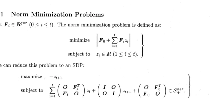
Let $F_{i}\in R^{q\cross r}(0\leq i\leq t)$. The

norm

minimization problem is defined

as:

minimize $||F_{0}+ \sum_{i=1}^{t}Fiz_{i}||$

subject to $z_{i}\in R(1\leq i\leq t)$.

$\}$

We

can

reduce this problem to

an

SDP:

maximize $-z_{t+1}$

subject to $\sum_{i=1}^{t}z_{i}+z_{t+1}+\in S_{+}^{q+r}$.

$\}$

Table 1 shows the performance comparisons

among

the $\dot{\mathrm{o}}\mathrm{r}\mathrm{i}\mathrm{g}\mathrm{i}\mathrm{n}\mathrm{a}\mathrm{l}$method (SDPA), the

conversion

method applied before solving with SDPA, and the completion method. As $q$ becomes larger, the

aggregate sparsity pattern and extended sparsity pattern becomes denser.

Table 1: Numerical results on norm minimization problems

In the

case

of norm minimization problems, the conversion

niethod

is better than the other

methods.

2.2

Quadratic

Programs

with Box Constraints

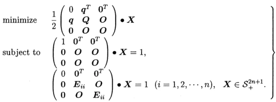
Let $Q\in S^{n}$ and $q\in R^{n}$. The quadratic program with box constraints is defined as: $\mathrm{m}\mathrm{i}\mathrm{n}\mathrm{i}\mathrm{m}\mathrm{i}\cdot \mathrm{z}\mathrm{e}$

$\frac{1}{2}x^{T}Qx+q^{T}x$

We have the following semidefinite programming relaxation of the above problem

minimize $\frac{1}{2}$ $\bullet$ $X$

subject to

$\cdot X=1$

,

$\bullet X=1(i=1,2, \cdots, n)$, $X\in S_{+}^{2+1}n$.

$\}$

Here $E_{ii}$ denotes the $n\cross n$ symmetric matrix with $(i, i)\mathrm{t}\mathrm{h}$ element 1 and all others $0$.

Table 2 shows the performance comparisons of these methods applied to this particular class

of problems. $\alpha$ denotes the sparsity of the objective function matrix. The entry “1001,1000” in

the$n$ column meansthat the primal matrix variable $X$ has block matrices of sizes $1001\cross 1001$ and

$1000\cross$1000.

Table 2: Numerical results

on

relaxation ofthe quadratic programs with box constraints

In the

case

of SDP relaxations of quadratic programs with box constraints, the completion

method is better than the other methods.

2.3

${\rm Max}$

-cut

Problem.s

over

Lattice

Graphs

Let $G=(V, E)$ be a lattice graph which is of size $k1\cross k2$ with a vertex set _{$V=\{1,2, ..., n\}$},

and

an

edge set $E=\{(i,j) : i,j\in V, i<j\}$

.

We assign

a

weight $C_{ij}=C_{ji}$ to each edge

$(i, j)\in E$

.

The maximum cut problem is to find a partition $(L, R)$ of $V$ that maximizes the cut

$c(L, R)=\Sigma_{i\in L},\in R{}_{ji}Cj\cdot$

Introducing.

a variable vector $u\in R^{n}$, we

can

,

$\mathrm{r}\mathrm{e}\mathrm{f}\mathrm{o}\mathrm{r}\mathrm{m}\mathrm{u}\mathrm{l}\mathrm{a}\mathrm{t}\mathrm{e}$ the problem as

a

nonconvex

quadratic program:

maximize $\frac{1}{2}\sum_{i<j}c_{ij}(1-u_{i}u_{j})$ subject to $u_{i}^{2}=1(1\leq i\leq n)$. $\}$

Here each feasible solution $u\in R^{n}$ of this problem corresponds to

a

cut $(L, R)$ with $L=\{i\in$

$V$ : _{$u_{i}=-1$}

}

and _{$R=\{i\in V : u_{i}=1\}$}. If

we

define $C$ to be the $n\cross n$ symmetric matrix with

by $A_{0}=\mathrm{d}\mathrm{i}\mathrm{a}\mathrm{g}(c_{e})-c$, where $e\in R^{n}$ denotesthevector of

ones

anddiag$(ce)$ the diagonal matrix

of the vector $Ce\in R^{n}$, we can obtain the following semidefinite programming relaxation of the

maximum cut problem:

minimize $-A_{0}$$\bullet$$X$

subject to $E_{ii}$ $\bullet$ $X=1/4(1\leq i\leq n),$ $X\in S_{+}^{n}$

.

$\}$

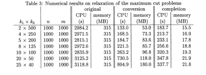
Table 3 compares the three algorithms for this problem. As $k1$ becomes larger, the aggregate

sparsity patterns remain

sparse,

but the extended sparsity pattern becomes denser.

Table 3: Numerical results on relaxation ofthe maximum cut problems

For the semidefinite programmingrelaxation ofmaximum cut problems

over

lattice graphs, the

conversion and the completion methods

are

better.

2.4

Semidefinite Programming Relaxation of Graph-partition

Problem

Let $G=(V, E)$ be

a

lattice graph which is of size $k1\cross k2$ with

a

vertex set _{$V=\{1,2, \ldots, n\}$}, and

an

edge set $E=\{(i,j) : i,j\in V, i<j\}$

.

We assign

a

weight $C_{ij}=C_{ji}$ to each edge $(i,j)\in E$.

We

assume

that $n$ is an

even

number. The graph partition problem is to find auniform partition

$(L, R)$ of$V,$ $i.e.$, apartition $(L, R)$ of$V$ with the same cardinality $|L|=|R|=n/2$, that minimizes

the cut $c(L, R)=\Sigma_{i\in LjR}\in c_{ij}$. This problem is formulated

as a

nonconvex

quadratic

program:

minimize $\frac{1}{2}\sum_{i<j}c_{ij}(1-uiu^{\backslash }j)$

subject to $(\Sigma_{i=1}^{n}u_{i})^{2}=0,$ $u_{i}^{2}=1(1\leq i\leq n)$.

As in themaximum cut problem,

we

can

derive

a

semidefinite programming relaxation of thegraph

partition problem:

minimize $A_{0}$$\bullet$ $X$

subject to $E_{ii}$$\bullet$ $X=1/4(1\leq i\leq n),$ $E\cdot X=0,$ $X\in S_{+}^{n}$.

$\}$ (6)

Here $A_{0}$ and $E_{ii}(1\leq i\leq n)$

are

the

same

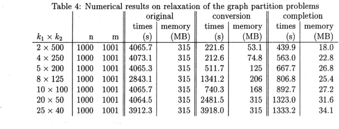
matrices as in the previous section, and $E$ denotes the $n\cross n$ matrix with all elements 1. Table 4 compares the three algorithms for this problem. As $k1$

Table 4: Numerical results on relaxation of the graph partition problems

becomes larger, the aggregate sparsity patterns remain sparse, but the extended sparsity pattern

becomes denser.

For the semidefinite programming relaxation of graph partition problems

over

lattice graphs,

the conversion and the completion methods

are

better.

3

Concluding

Remarks

In this article,

we

explained the mechanisms of the completion method. Next

we

presented some

numerical results which compared the original method, the conversion method and the completion

method. As a result, we confirmed the effectiveness of the conversion method and the completion

method.

References

[1] F. ALIZADEH, J.-P. A. HAEBERLY AND M. L. OVERTON, Primal-dual interior-point

meth-ods

_f.or

_semidefinite

programming: convergence rates, stability and numerical results, SIAM J.

Optim., 8 (1998), pp.

746-768.

[2] K. FUJISAWA, M. KOJIMA AND K. NAKATA, SDPA (Semidefinite Programming Algorithm)

–User’s Manual –, Technical Report B-308, Department of Mathematical and

Comput-ing Sciences, Tokyo Institute of Technology, Japan, December 1995 (revised August 1996).

Available at $\mathrm{f}\mathrm{t}\mathrm{p}://\mathrm{f}\mathrm{t}\mathrm{p}.\mathrm{i}\mathrm{s}.\mathrm{t}\mathrm{i}\mathrm{t}\mathrm{e}\mathrm{c}\mathrm{h}.\mathrm{a}\mathrm{C}.\mathrm{j}\mathrm{p}/\mathrm{p}\mathrm{u}\mathrm{b}/\mathrm{O}\mathrm{p}\mathrm{R}\mathrm{e}\mathrm{s}/\mathrm{s}\mathrm{o}\mathrm{f}\mathrm{t}\mathrm{W}\mathrm{a}\mathrm{r}\mathrm{e}/\mathrm{S}\mathrm{D}\mathrm{P}\mathrm{A}$ .

[3] M. FUKUDA, M. KOJIMA, K. MUROTA AND K. NAKATA, Exploiting sparsity in

semidefinite

programming via matrix completion I.. general framework, SIAM J. Optim., to appear.

[4] C. HELMBERG, F. RENDL, R. J. VANDERBEI AND H. WOLKOWICZ, An interior-point

method

_for

_semidefinite

programming, SIAM J. Optim., 6 (1996), pp. 342-361.

[5] M. Kojima, M. Shida and

S.

Shindoh, “Search directions in the

SDP

and themonotone

SDLCP:

[6] M. Kojima, S. Shindoh and S. Hara, $‘(\mathrm{I}\mathrm{n}\mathrm{t}\mathrm{e}\mathrm{r}\mathrm{i}\mathrm{o}\mathrm{r}$-point methods for the monotone semidefinite

linear complementarity problems,”

SIAM

Journal on Optimization 7 (1997) 86-125.

[7] R. D. C. MONTEIRO, Primal-dual path-following algorithms

_{for semidefinite}

programming,

SIAM

J. Optim., 7 (1997), pp.

663-678.

[8] R.D.C. Monteiro and Y. Zhang, (‘A _{unified analysis for} a class of path-following

primal-dual interior-point algorithms for semidefinite programming,” Mathematical Programming 81

(1998)

281-299.

[9] Yu. E. NESTEROV AND M. J. TODD, Primal-dual interior-point methods

for self-scaled

cones,

SIAM J. Optim., 8 (1998), pp.

324-364.

[10] M.J. Todd, K.C. Toh and R.H. T\"ut\"unc\"u, $‘(\mathrm{O}\mathrm{n}$ the

Nesterov-Todd

direction in semidefinite

programming,” Technical Report, School of Operations Research and Industrial Engineering,

Cornell University, Ithaca, New York 14853-3801, USA, March 1996, Revised May 1996, to