複素対称行列を係数に持つ一般化シフト線形方程式の高速数値解法 (数値解析と数値計算アルゴリズムの最近の展開)

A fast numerical method for

generalized

shifted

linear

systems

with

complex symmetric

matrices

(

_{複素対称行列を係数に持つ一般化シフト線形方程式の高速数値解法}

)

愛知県立大学 曽我部知広 (Tomohiro Sogabe)

Aichi Prefectural University

鳥取大学 星健夫 (Takeo Hoshi)

Tottori University

名古屋大学 張紹良 (Shao-Liang Zhang)

Nagoya University

東京大学 藤原毅夫 (Takeo Fujiwara)

The University of Tokyo

Abstract

We consider the solution of generalized shifted linear systems with complex

symmetric matrices. We present a numerical method for solving the linear systems

basedontheshiftedCOCG method withasuitable bilinear form. The methodcan

be attractive when the inner linear systems can efficiently be solved.

1

Introduction

We consider the solution of generalized shifted linear systems with complex symmetric

(non-Hermitian) matrices of the form:

$(A+\sigma_{\ell}B)x^{(t)}=b$, _$P=1,2,$

$\ldots,$$m$, (1.1)

wherethecoefficient matrices$L(\sigma_{l})$ $:=A+\sigma_{\ell}B$ arenonsingular$N\cross N$complex symmetric

sparse matrices, i.e., $L(\sigma_{p})=L(\sigma_{\ell})^{T}\neq\overline{L}(\sigma_{1})^{T}$, with scalar shifts $\sigma_{l}\in C,$ $I$ is the

$N\cross N$ identity matrix, and $x^{(\ell)},$$b$

are

complex vectors of length $N$. Matrices $A$ and $B$

are

assumed to be nonsingular. The linear systems (1.1) arise in large scale electronic

structure theory, and there is

a

strong need for fast solution of the linear systems.

When the coefficient matrices $L(\sigma_{p})$ of the linear systems (1.1)

are

real symmetric

matrices, the linear systems

are

known

as

parametrized (real) symmetric linear systems.

An efficient numerical method for solving the linear systemshas been proposed by

Meer-bergen [6]. For studies

on

other parametrized linear systems, see, e.g.,

an

excellent survey

by Simoncini

&

Szyld [8].

When thematrix $B$ is the identitymatrix, the linear systems (1.1) reduce to standard

shifted linear systems with complex symmetric matrices. Efficient numericalmethods for

this class of shifted linear systems have been studied based on Krylov subspace methods

such

as

the shifted QMR method [3], the shifted WQMR method [9], and the shifted

COCG method [10].

In this paper,

we

extend the shifted

COCG

method in order to solve the generalized

into standard shifted linear systems and (ii) using

a

suitable bilinear form in order to

make

use

ofproperties of thematrices $L(\sigma_{l})$.

This paperis organized

as

follows. The algorithm and apropertyof the shiftedCOCG

method for solvingshifted linear systems with complexsymmetric matrices are described

in the next section. Then, in Section 3, an extension of the shifted COCG method is

proposed for solving the generalized shifted linear systems. Results

on

some numerical

experiments

are

reported in Section 4. Finally,

some

concluding remarks

are

made in

Section 5.

2

The shifted

COCG

method

Theshifted COCGmethod [10] is

a

powerfulsolverfor shifted linear systems with complex

symmetric matrices of the form:

$(A+\sigma_{f}I)x^{(l)}=b$, _$P=1,2,$

$\ldots,$$m$. (2.1)

Let $x_{0}^{(\ell)}$ be the initial approximate solutions for the linear systems (2.1) so that the

corresponding initialresidual vectors$r_{0}^{(\ell)}$ $:=b-(A+\sigma_{\ell}I)x_{0}^{(\ell)},$ $P=1,2,$

$\ldots,$$m$arecollinear,

i.e., thereexist $c_{2},$$c_{3},$

$\ldots,$$c_{m}\in C$ such that

$r_{0}^{(1)}=c_{2}r_{0}^{(2)}=$ . . . $=c_{m}r_{0}^{(m)}$.

Then, the shifted COCG method finds approximate solutions of (2.1) over the following

affine space:

$x_{n}^{(l)}\in x_{0}^{(\ell)}+K_{n}(A+\sigma_{\ell}I, r_{0}^{(p)})$ (2.2)

so

that the nth residual vector $r_{n}^{(\ell)}$ $:=b-(A+\sigma_{\ell}I)x_{n}^{(l)}$ satisfies

$r_{n}^{(\ell)}\in K_{n+1}(A+\sigma_{l}I, r_{0}^{(p)})\perp K_{n}(\overline{A+\sigma_{\ell}I}, \overline{r}_{0}^{(l)})$. (2.3)

Here $K_{n}(A, b)$ is n-dimensional Krylov subspace given by span$\{b, Ab, . . . , A^{n-1}b\}$. Since

$r_{0}^{(l)\prime}s$ are collinear, it is widely known that shift-invariance property of Krylov subspaces

holds, i.e.,

$K_{n}(A+\sigma_{i}I, r_{0}^{(i)})$ $=$ $K_{n}(A+\sigma_{j}I, r_{0}^{(j)})$,

$K_{n}(\overline{A+\sigma_{i}I}, \overline{r}_{0}^{(i)})$ _$=$ $K_{n}(\overline{A+\sigma_{j}I}, \overline{r}_{0}^{(j)})$

for all $i,j=1,2,$$\ldots,$$m$. This

means

that it is enough to generate only

one

Krylov

$f\circ rsimp1icityx_{0^{p}}^{(\ovalbox{\tt\small REJECT}_{=0,isdescribedasfo11ows:}^{tocostefficienta1gorithm.T}}Subspace,1eadin$ healgorithm of the shiftedCOCG

Algorithm 1: Shifted COCG

$x_{0}^{(\ell)}=p_{-1}^{(\ell)}=0,$ _{$r_{0}=b$},

$\beta_{-1}=0_{\dot{}}\pi_{0}^{(s,\ell)}=\pi_{-}^{(s}i^{l)}=\alpha_{-1}=1$,

for $n=0,1,$$\ldots$ until $\Vert r_{n}\Vert_{2}\leq\epsilon\Vert b\Vert_{2}$ do:

$p_{n}=r_{n}+\beta_{n-1}p_{n-1}$,

$\alpha_{n}=\frac{(r_{n},r_{n})}{(p_{n},(A+\sigma_{s}I)p_{n})}$,

$x_{n+1}=x_{n}+\alpha_{n}p_{n}$,

(begin shifted system)

for $P(\neq s)=1,$_$\ldots,$$m$ if$\Vert r_{n}^{(l)}\Vert_{2}>\epsilon\Vert b\Vert_{2}$ then,

$\pi_{n}^{(s}\dotplus_{1}^{\ell)}=R_{n+1}^{(s)}(\sigma_{s}-\sigma_{\ell})arrow(2.4)$ $\beta_{n-1}^{(\ell)}=(\frac{\pi_{n-1}^{(s,\ell)}}{\pi_{n}^{(s,\ell)}})^{2}\beta_{n-1}$, $\alpha_{n}^{(l)}=\frac{\pi_{n}^{(s,l)}}{\pi_{n}^{(s}\dotplus_{1}^{\ell)}}\alpha_{n}$, $p_{n}^{(l)}= \frac{1}{\pi_{n}^{(s,\ell)}}r_{n}+l^{i_{n-1}^{(p)}p_{n-1}^{(\ell)}}$, $x_{n+1}^{(\ell)}=x_{n}^{(\ell)}+\alpha_{n}^{(\ell)}p_{n}^{(\ell)}$ , end if end

(end shifted system)

$r_{n+1}=r_{n}-\alpha_{n}(A+\sigma_{s}I)p_{n}$,

$\beta_{n}=\frac{(r_{n+1},r_{n+1})}{(r_{n},r_{n})}$

.

end

Herethe symbol $(x, y)$ bethebilinear formgiven by$x^{T}y$, which isdifferent from standard

dot product $x^{H}y$

.

In Algorithm 1, the computational formula for $\pi_{n}^{(s}\dotplus^{p_{1}}$) is given below.

$R_{n}^{(s)}( \lambda)=(1-\alpha_{n-1}^{(s)}\lambda)R_{n-1}^{(s)}(\lambda)+\frac{\beta_{n-2}^{(s)}}{\alpha_{n-2}^{(s)}}\alpha_{n-1}^{(s)}(R_{n-1}^{(s)}(\lambda)-R_{n-2}^{(s)}(\lambda)),$$n=2,3,$

$\ldots$, (2.4)

3

An

extension

of the

shifted

COCG

method

to

the

generalized shifted linear

systems

In this section,

we

extend the shifted

COCG

method for solving the generalized shifted

linear systems (1.1). We first transform the generalized shifted linear systems (1.1) into

the following form:

$(B^{-1}A+\sigma_{l}I)x^{(\ell)}=B^{-1}b$, $\ell=1,2,$$\ldots,$$m$

.

(3.1)

The above linear systems

are

well-known (standard) shifted linearsystems. It is

therefore

natural to

use

Krylov subspace methodsfor non-Hermitian shifted linear systems such

as

the shiftedGMRES method by Datta

&

Saad [1] and the shifted BiCGStab$(\ell)$ method by Frommer [4]. For other methods to solve non-Hermitian shifted linear systems, see, e.g.,

[8]. These methods however does not

use

the property of $L(\sigma_{\ell})$, i,e, complex symmetric

matrices. This motivates

us

to find algorithm that makes

use

of the property, and

we

will show that the algorithm has nice properties: short-term

recurrence

relation and

no

requirement of restarting.

We

now

extend the shifted COCG method to the generalized shifted linear systems

(1.1). We consider finding approximate solutions over the following affine space:

$x_{n}^{(l)}\in x_{0}^{(l)}+K_{n}(B^{-1}A+\sigma_{\ell}I, B^{-1}r_{0}^{(\ell)})$ (3.2)

so that the nth residual vector $r_{n}^{(\ell)}$ $:=b-(B^{-1}A+\sigma_{\ell}I)x_{n}^{(p)}$ satisfies

$r_{n}^{(\ell)}\in K_{n+1}(B^{-1}A+\sigma_{l}I, B^{-1}r_{0}^{(\ell)})\perp\overline{B}K_{n}(\overline{B^{-1}A+\sigma_{\ell}I},\overline{B}\overline{r}_{0}^{(l)})1$ . (3.3)

It is easy to

see

that the strategy $(3.2)-(3.3)$ _{is equivalent} to the strategy $(2.2)-(2.3)$ of

the shifted COCG method when the matrix $B$ is the identity matrix.

This strategy corresponds to applying the shifted COCG method with the following

bilinear form:

$(x, y)_{B}:=x^{T}By$

.

(3.4)

tothe shifted linear systems (3.1). The resulting algorithm, referred to

as

the generalized

shifted COCG method, is given next.

$x_{0}^{(l)}=p_{-1}^{(\ell)}=0,$ _{$r_{0}=b$},

$\beta_{-1}=0,$ $\pi_{0}^{(s,\ell)}=\pi_{-}^{(s}i^{l)}=\alpha_{-1}=1$,

for $n=0,1,$$\ldots$ until $\Vert r_{n}\Vert_{2}\leq\epsilon\Vert b\Vert_{2}$ do:

$p_{n}=B^{-1}r_{n}+\beta_{n-1}p_{n-1}$,

$x_{n+1}.arrow-\backslash x_{n}\cdot+\alpha_{n}p_{n}$,

(beginshifted system)

For $\ell(\neq s)=1,$_$\ldots,$$m$

if $\Vert r_{n}^{(\ell)}\Vert_{2}>\epsilon\Vert b\Vert_{2}$ then,

$\pi_{n+1}^{(s,\ell)}=R_{n+1}^{(s)}(\sigma_{s}-\sigma_{\ell})arrow(2.4)$ $\beta_{n-1}^{(\ell)}=(\frac{\pi_{n-1}^{(s,\ell)}}{\pi_{n}^{(s,\ell)}})^{2}\beta_{n-1}$, $\alpha_{n}^{(p)}=\frac{\pi_{n}^{(,p)}s}{(s,p)}\alpha_{n}$ , $\pi_{n+1}$ $p_{n}^{(\ell)}= \frac{1}{\pi_{n}^{(s,\ell)}}B^{-1}r_{n}+\beta_{n-1}^{(\ell)}p_{n-1}^{(\ell)}$, $x_{n+1}^{(\ell)}=x_{n}^{(\ell)}+\alpha_{n}^{(\ell)}p_{n}^{(\ell)}$, end if end

(end shifted system)

$r_{n+1}=r_{n}-\alpha_{n}(A+\sigma_{\delta}B)p_{n}$,

$\beta_{n}=\frac{r_{n+1}^{T}B^{-1}r_{n+1}}{r_{n}^{T}B^{-1}r_{n}}$

.

end

It is worth mentioning that Algorithm 2 generates original residual vectors, i.e., $r_{n}=$

$b-(A+\sigma_{s}B)x_{n}$. In Algorithm 2, the computational formulafor $\pi_{n}^{(s}\dotplus^{\ell_{1}}$) is given below.

$R_{n}^{(s)}( \lambda):=(1-\alpha_{n-1}^{(s)}\lambda)R_{n-1}^{(s)}(\lambda)+\frac{\beta_{n-2}^{(s)}}{\alpha_{n-2}^{(s)}}\alpha_{n-1}^{(s)}(R_{n-1}^{(s)}(\lambda)-R_{n-2}^{(s)}(\lambda))$, (3.5)

where $R_{t}^{(s)}(\lambda)=1,$ $R_{1}^{(s)}(\lambda)=(1-\alpha_{0}\lambda)R_{0}^{(s)}(\lambda)$

.

Here

we

note that in Algorithm 2,

we

need to compute $B^{-1}r_{n}$ that is equivalent to finding the solution_{$y_{n}$} of the linear systems

of the form:

$By_{n}=r_{n}$ (3.6)

at each iteration step. Since thematrix $B$is real symmetric positive definite, the systems

could be solved by the CG method with

a

suitable preconditioner.

In what follows, the linear systems (3.6) and the solutions

are

referredto

as

innerlinear

systems and inner solutions, respectively. The linear systems (1.1) and the solutions $x_{n}$

are

referred to

as

outer linear systems and outer solutions, respectively.

On

a

derivation of the generalized shifted COCG method

Bi-CG method [4]. Applying theshifted Bi-CG method to the linear systems (3.1) yields

$x_{n}^{(1)}\in x_{0}^{(\ell)}+K_{n}(B^{-1}A+\sigma_{l}I, B^{-1}r_{0}^{(l)})$, (3.7) $r_{n}^{(\ell)}\in K_{n+1}(B^{-1}A+\sigma_{\ell}I, B^{-1}r_{0}^{(\ell)})\perp K_{n}((B^{-1}A+\sigma_{\ell}I)^{H}, r_{0}^{*(\ell)})$, (3.8)

where $r_{0}^{*(\ell)}$

are

so-called shadow vectors. If

we

choose $r_{0}^{*(l)}=\overline{r}_{0}^{(l)}$, then it followsthat

$K_{n}((B^{-1}A+\sigma_{p}I)^{H}, r_{0}^{*(l)})$ _$=$ $K_{n}((B^{-1}A+\sigma_{\ell}I)^{H}, (\overline{B})(\overline{B})^{-1}\overline{r}_{0}^{(\ell)})$

$=$ $K_{n}((\overline{AB^{-1}+\sigma_{l}I}), (\overline{B})(\overline{B})^{-1}\overline{r}_{0}^{(\ell)})$

$=$ $K_{n}(\overline{AB}1, (\overline{B})(\overline{B})^{-1}\overline{r}_{0}^{(p)})$ $=\overline{B}K_{n}(\overline{B}\overline{A},\overline{B}\overline{r}_{0}^{(1)})$

$=\overline{B}K_{n}(\overline{B^{-1}A+\sigma_{l}I}, \overline{B}\overline{r}_{0}^{(l)})1$.

From which, we see that the strategy $(3.7)-(3.8)$ of the shifted Bi-CG method with the

choice $r_{0}^{*(l)}=\overline{r}_{0}^{(\ell)}$is equivalent to the strategy $(3.2)-(3.3)$ ofthe generalized shiftedCOCG

method. This result

means

that the generalized shifted COCGmethod is asimplification

of the shifted Bi-CG method applied to the linear systems (3.1).

This relationessentiallygoes back to the relation between the

Bi-CG method

and the

COCG

method that has elegantly been shown by Freund [2].

A seed switching technique for the generalized shifted COCG method

From the property $r_{n}^{(s)}=\pi_{n}^{(s,\ell)}r_{n}^{(\ell)}$ it follows that $\Vert r_{n}^{(l)}\Vert\leq\Vert r_{n}^{(s)}\Vert$ if $|\pi_{n}^{(s,\ell)}|=|R_{n}^{(s)}(\sigma_{s}-$

$\sigma_{l})|\geq 1$

.

Hence, if one could find a seed system such that $|R_{n}^{(s)}(\sigma_{s}-\sigma_{\ell})|\geq 1$ for all

$\ell$, then all shifted systems could be solved. In practice, it is generally hard to find

such linear system in advance because it

means

to find the system with the slowest

convergence behavior. For the generalized shifted COCG method,

we

have developed

the seed switching technique in order to avoid the problem [7]. See also [11] for

one

of

the applications. This technique can also be applied to the generalized shifted COCG

method, and the resulting technique is summarized

as

follows:

1. Choose

a

seed system, and then start Algorithm 2;

2. If the seedsystem

was

solved at nth iteration, then find the new one;

3. Start Algorithm 2 from $(n+1)$th iteration using the new seed system.

In II, as oneofcriteriaforchoosingthenewseed system$\overline{s}$, weadopt _{$\tilde{s}=\arg\max_{i\in S}\{\Vert r_{n}^{(\ell)}\Vert\}$},

where $S$ denotes an index set of unsolved systems. In III,

we

need two steps to switch

the old seed system to the new one. First, compute

$\pi_{n}^{(s}\dotplus^{\overline{s}_{1})}=R_{n+1}^{(s)}(\sigma_{s}-\sigma_{\tilde{s}})$_, $\beta_{n}^{(\tilde{s})}=(\pi_{n}^{(s,\tilde{s})}/\pi_{n}^{(s}\dotplus^{\tilde{s}_{1})})^{2}\beta_{n}$

for obtaining $r_{n+1}^{(\tilde{s})}$ and $\beta_{n}^{(\tilde{s})}p_{n}^{(\tilde{s})}$, and then

we

have $p_{n+1}^{(\tilde{s})}(=B^{-1}r_{n+1}^{(\tilde{s})}+\beta_{n}^{(\tilde{s})}p_{n}^{(\tilde{s})})$

.

Now,

$(B^{-1}A+\sigma_{\tilde{s}}I)x^{(\tilde{s})}=B^{-1}b$ from $(n+1)$th iteration step. Second, to solve the rest of

systems by using the

new

seed $\tilde{s}$, it requires generating $\alpha_{n+1}^{(\ell)},$ $\beta_{n}^{(\ell)}$ from the

new

seed.

They

can

be readily generated by the following polynomial:

$\pi_{n}^{(\tilde{s}}\dotplus_{1}^{\ell)}=R_{n+1}^{(\tilde{s})}(\sigma_{\tilde{S}}-\sigma_{\ell})$ for all $p\in S$

.

To obtain the above polynomial,

we

need to compute

$\alpha_{i}^{(\tilde{s})}=(\pi_{i}^{(s,\tilde{s})}/\pi_{i+1}^{(s,\tilde{s})})\alpha_{\ell_{arrow}}$. $\beta_{j}^{(\tilde{\epsilon})}=(\pi_{j}^{(\epsilon,\tilde{s})}/\pi_{j+1}^{(s,\tilde{s})})^{2}\beta_{j}$

for $i=0,$$\ldots,$$n,$ $j=0,$ $\ldots,$$n-1$

.

Hence, the switching strategy requires only scalar

operations, and

moreover

we

see

that if breakdown does not occur, iteratingthe process

from (II) to (III) enables

us

to keep solving the systems without losing the dimension of

the Krylov subspace that has been generated until thelast switching.

The results of

some

numerical experiments will be reported in order to show the

practical efficiency of the generalized shifted COCG method.

4

Numerical

examples

In thissection, we report on

some

numerical examples concerning the generalized shifted

COCG method (Algorithm 2). Alltests

were

performed

on a

workstation with

a

2.$6GHz$

AMD Opteron(tm) processor 252 using double precision arithmetic. Codes

were

written

in Fortran 77 and compiled with g77-O3. In all

cases

the stopping criteria

were

set

as

$\epsilon=10^{-12}$

.

The inner linear systems (3.6)

was

solved by the CG method without

preconditioner that is

more

efficient than IC(0) in

our

problems. The

CG

method

was

stopped when its relative residua12-norm becomes less than

or

equal to the given value

$\epsilon_{CG}$, and in

our

numerical example

we

used $\epsilon_{CG}=10^{-6},10^{-8},10^{-10},10^{-12}$

.

4.1

Example

1

Thefirst problem

comes

from theelectronic structurecomputationof

Au

with

256

atoms,

which is written.as follows:

$(\sigma_{f}S-H)x^{(l)}=e_{1}$, _$P=1,2,$

$\ldots$, 1001,

where $\sigma_{p}=0.400+(P-1+i)/1000,$ $S,$ $H\in R^{2304\cross 2304}$

are

asymmetric positive definite

matrix and

a

symmetric matrix with 1,059,584 entries, $e_{1}=(1,0, \ldots, 0)^{T}$

.

Since the

generalized shifted COCG method requires the choice ofa seed system,

we

have chosen

the optimal seed $(\ell=174)$ in this problem; otherwise

some

linear systems would remain

$\frac{\simeq=\Phiarrow\varpi 0\subset\omega}{\tilde{\vec{\supseteqq\in}\Phi}\circ}$

$O$ $2OO$ $4OO$ $6OO$ SOO $100O$ Index of the shifted linear systems(1)

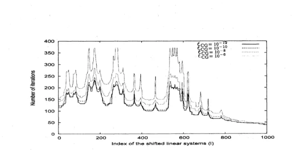
Figure 1: Number of iterations for the generalized shifted COCG method

versus

theindex

of the shifted linear systems for example 1.

$O$ $2OO$ $4OO$ $6O0$ SOO $1OOO$

lndex of the shifted linear systemS(1)

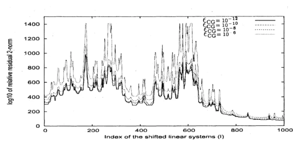
Figure 2: The dependence of the true relative residua12-norm

on

the accuracy of the

Figure 1 shows the dependency of required number of iterations for the generalized

shifted COCG method on the accuracy of inner solutions (3.6). From Fig.1, the

more

accurate

we

solve the inner linear systems, the less number of iterations

were

required.

Since

the inner linear systems

are

solved roughly,

we

need to check the loss of

accuracy

of the outer solutions. So,

we

next show the dependency of the

accuracy

for the outer

solutions of (1.1) on the accuracy of inner solutions of (3.6) in Fig.2. We

see

in Fig. 2

that the accuracy is almost the

same

order

as

that of the inner solutions. This example

implies how robust the present algorithm is

even

if

we

solve the inner solutions roughly.

The CPU time of the generalized shifted COCG method is given in Table 1. From

Table 1, we see that roughly solving inner linear systems does not always lead to

time-efficient, this is because total number of iterations for tlie seed systelntended to increase,

see

Fig. 1.

The results using the seed switching technique

are

described in Table 2. In Table 2,

470 linear systems remained unsolved after the generalized shifted COCG method with

the initial seed $0.400+0.001i$

was

solved, which

can

be a practical issue. Using the seed

switching technique, it automatically chose thesecond seed$0.573+0.001i$, and

as

a

result

all linear systems

were

solved. Next,

we

chose the initial seed $1.400+0.001i$

.

Then, the

switchrequiredthree times. Intwocases, the last seedvalues

were same.

We have checked

that when

we

used the last seed value,

no

switch occured during the iterations for solving

all linear systems. In

our

numericalexperiments, the number of switching actions was, at

most, three. In terms of CPU time, the generalized shifted COCG using seed switching

technique required 33.70

sec.

with the initial seed $0.400+0.001i$ and

34.30

sec.

with

the initial seed $1.400+0.001i$, where $\epsilon_{CG}=10^{-12}$

.

Finally, the CPU time ofthe

COCG

method applied to all shifted linear systems

was

1217.3

sec.

We also used the

COCG

method with IC(0)-type _{preconditioner, but it did not improve the performance due to}

large number of incompletefactorizations.

Table 1. CPU time required for solving generalized shifted linear systems for example 1.

Table 2. Results on the generalized shifted COCG method

4.2

Example

2

The second problem is larger than the first problem, which

comes

from the electronic

structure computation of Au with 864 atoms:

$(\sigma_{\ell}S-H)x^{(\ell)}=e_{1\dot{)}}$ _$\ell=1,2,$

$\ldots$, 1001,

where $\sigma_{\ell}=0.400+(P-1+i)/1000,$ $S,$ $H\in R^{7776\cross 7776}$

are a

symmetric positive definite

matrix and asymmetric matrixwith 3,619,104 entries. Other conditions are the

same

as

in example 1. From Figs. 3 and 4, we

see

similar tendency to that shown in example 1.

$\frac{rightarrow\overline{\approx\varpi\supset}}{arrow\infty\omega}\Subset\subset 0$

’

$\underline{\frac{\Leftrightarrow}{rightarrow 0}\frac{=\varpi}{arrow\sim\omega}\Phi\circ>}$

Figure

3:

Number of iterations for the generalized shifted COCG method

versus

theindex

of the shifted linear systems for example 2.

Figure 4: The dependence of the true relative residua12-norm on the accuracy of the

The

CPU

time of the generalized

shifted COCG

method is given in Table

3. From

Table 3, the most time-consuming part

was

to solve the seed system. So, it is worth

reducingthe CG iterations by

a

sophisticated preconditioner. In the case, it alsofoundto

be better to

use

more

accurate criterion for the inner solutions. The number ofswitching

actions was, atmost,two. In termsofCPUtimeinTable 4, The generalized shiftedCOCG

usingseed switching technique required522.0

sec.

with the initial seed $0.400+0.001i$and

525.7

sec.

with the initial seed $1.400+0.001i$, where $\epsilon_{CG}=10^{-12}$

.

Finally,

we

note that the CPU time of the

COCG

method without preconditioning,

which was better than IC(0)-type preconditioning, applied to all shifted linear systems

was

16867.8

sec.

Table 3.

CPU

time required for solving generalized shifted linear systems for example 2.

Table 4. Results

on

the generalized shifted

COCG

method

using seed switching technique for example 2.

5

Conclusion

In this paper, the shifted

COCG

method

was

extended to solving generalized shifted

linear systems with complex symmetric matrices. The resulting algorithm, the generalized

shifted COCG method, was derived from two different ways: (1) the shifted COCG

method with a bilinear form and (2) a simplification of the shifted Bi-CG method. We

have learned that in

our

numericalexamples,

we can use

iterativemethods for solving the

inner linear systems, and the accuracyof the solutions depends linearlyonthe accuracyof

the solutions for the inner linear systems. From numerical examples, the algorithm found

to be highly attractive when the inner linear systems canefficiently be solved. Since the

present strategy

can

also be applied to the shifted QMR method and the shifted WQMR

method, the comparison among them will be

our

future work.

The generalizedshifted

COCG

methodhas already been implemented in the quantum

mechanical nanomaterial simulation code ‘ELSES’ $($http:$//www.elses.jp)$ and willbe

ap-plied to various nanomaterials

as

interdisciplinary research between applied mathematics

Acknowledgement

This work

was

partially supported by KAKENHI (Grant No. 21760058).

References

[1] B. N. Datta and Y. Saad, Arnoldi methods for large Sylvester-like observer matrix

equations, and

an

associated algorithm for partial spectrum assignment, Linear

Al-gebra Appl., 154-156 (1991), pp. 225-244.

[2] R. W. Freund, Conjugate gradient-type methods for linear systems with complex

symmetric coefficient matrices, SIAM J. Sci. Stat. Comput., 13 (1992), pp. 425-448.

[3] R. W. Freund, Solution of shifted linear systems by quasi-minimal residual

itera-tions, Numerical Linear Algebra, L. Reichel, A. Ruttan, and R. S. Varga eds., W. de

Gruyter, (1993), pp. 101-121.

[4] A. Frommer, BiCGStab$(\ell)$ for families of shifted linear systems, Computing, 70

(2003), pp. 87-109.

[5] T. Fujiwara, S. Yamamot$0$, T. Hoshi, S. Nishino, H.Teng, T. Sogab$e$,

S.-L.

Zhang,

M. Ikeda, M. Nakashima, N. Watanabe, Large-scale Electronic

Structure

Calculation

Theory and Applications, Preprint; http:$//arxiv.org/abs/1002.1202$

[6] K. Meerbergen, The solution of parametrized symmetric linear systems, SIAM J.

Matrix Anal. Appl., 24 (2003), pp. 1038-1059.

[7] T. Sogabe, T. Hoshi, S.-L. Zhang, and T. Fujiwara, A numerical method for

cal-culating the Green$s$ function arising from electronic structure theory, in: Frontiers

of Computational Science, eds. Y. Kaneda, H. Kawamura and M. Sasai,

Springer-Verlag, Berlin/Heidelberg, 2007, pp. 189-195.

[8] V. Simoncini and D. B. Szyld, Recent computationaldevelopments in Krylov

Sub-space Methods for linear systems, Numer. Linear Algebra Appl., 14 (2007), pp. 1-59.

[9] T. Sogabe, T. Hoshi, S.-L. Zhang, and T. Fujiwara, On

a

weighted quasi-residual

minimization strategy of the QMR method for solving complex symmetric shifted

linear systems, Electron. Trans. Numer. Anal., 31 (2008), pp. 126-140.

[10] R. Takayama, T. Hoshi, T. Sogabe, S.-L. Zhang, and T. Fujiwara, Linear algebraic

calculation ofGreen$s$ function for large-scale electronic structure theory, Phys. Rev.

$B73$, 165108 (2006), pp. 1-9.

[11] S. Yamamoto, T. Sogabe, T. Hoshi, S.-L. Zhang, and T. Fujiwara, Shifted COCG

method and its application to double orbital extended Hubbardmodel, J. Phys. Soc.