Large-amplitude solitary waves on a linear shear current (Workshop on Nonlinear Water Waves)

全文

(1)9. Large‐amplitude solitary waves on a linear shear current. Sunao Murashige Department of Mathematics and Informatics, Ibaraki University. Abstract. This work considers two‐dimensional steady motion of solitary waves progressing in permanent form with constant speed on a shear current of which the horizontal velocity varies linearly with depth. In particular, we focus on peaking of the wave crest with increase of amplitude. First, local flow analysis near the crest of the peaked wave using conformal mapping determines singularities of solutions at the wave crest. It is shown that the inner angle of the corner at the crest of the peaked wave does not depend on the magnitude of shear current. Next,. solutions of the two long wave models, the Korteweg‐de Vries (KdV) model and the strongly nonlinear model, for solitary waves on a linear shear current are numerically compared with those the full Euler system. Numerical examples demonstrate that these long wave models can qualitatively capture variation of peaking phenomenon with the magnitude of shear current. In addition, linear stability analysis of steady solutions of solitary waves is discussed using the two long wave models.. 1. Introduction. Some previous works have shown that motion of surface waves may be affected by shear currents varying with depth, which are caused by wind stresses at the water surface or. frictional stresses acting on the bottom (for example [13, §4]). For two‐dimensional motion of incompressible and inviscous fluid, assumption of linear variation of the horizontal velocity of a shear current with depth allows us to formulate the problem within the framework of irrotational wave theory. In this work, we consider large‐amplitude motion of solitary waves propagating on a linear shear current, as shown in fig. 1. On the assumption. of linear shear current, Teles da Silva & Peregrine [16], Pullin & Grimshaw [14] and Vanden‐Broeck [17] demonstrated some interesting nonlinear phenomena in solitary wave motion using numerical computation of the full Euler system. Among them, we focus on peaking phenomenon, namely peaking of the wave crest with increase of amplitude, as shown fig.2. Crest singularities of the peaked wave can be investigated using local flow analysis near. the wave crest, similarly to the case without shear current [7] [15, p.225]. In section 2.3, it will be shown that conformal mapping of the flow domain to a suitable complex plane helps us examine high‐order singularities. Some computed results of wave profiles in fig.2 show that solitary waves on a linear shear current can attain peaked waves with small amplitude. This indicates that existence.

(2) 10 of a shear current may change the breaking limit of surface waves. For systematic under‐ standing of this, we introduce the two long wave models, the Korteweg‐de Vries (KdV). model [1, 6] and the strongly nonlinear model [4] in section 3. It may be worthwhile to investigate linear stability of steady solutions of these long wave models, as a preliminary work for elucidation of the mechanism of generation of wave breaking. It should be noted that linear stability of steady solutions of water waves on a linear shear current has bee. numerically investigated for periodic waves [5, 12], but not for solitary waves.. h). h). (a) Upstream propagation (\Omega>0). Fig.1. A solitary wave on a linear shear current.. \frac{y}{h}. \Omega. : the shear strength.. \frac{y}{h}. (a). \Omega^{*}=0. \frac{y}{h}. ( b). \Omega^{*}=-0.2. ( d). \Omega^{*}=-0.6. \frac{y}{h}. (c). Fig.2. (b) Downstream propagation (\Omega<0). \Omega^{*}=-0.4. Wave profiles of a solitary wave on a linear shear current. \Omega^{*}=\Omega h/\sqrt{gh}. Solutions of the full Euler system are numerically obtained using the boundary. integral method [17]..

(3) 11 11. 2 2.1. Steady solutions of the full Euler system Representation of solutions using the complex velocity potential. Consider a left‐going solitary wave on a linear shear current in the frame of reference moving with wave speed c , as shown in fig. 1. Assume that a fluid is incompressible and inviscid, and that fluid motion is two‐dimensional and steady in the vertical cross‐section along the progressing direction of wave. The horizontal velocity of a linear shear current is given by U_{0}=\Omega(y+h) where the shear strength \Omega and the water depth h are both constant. Then the total velocity vector (U, V) can be split into the velocity of a linear shear current and that of wave motion as. (\begin{ar y}{l U V \end{ar y}) and its vorticity. \omega. +_{w\tilde{a}(\begiven{ar y}{l motu v \end{air oy})n. =. (1). is given by. \omega=V_{x}-U_{y}=-\Omega(= constant). (2). For two‐dimensional motion of incompressible and inviscid fluid, the vorticity is conserved, and then the velocity vector (u, v) satisfies. (3). v_{x}-u_{y}=0. Thus the perturbed flow due to wave motion is irrotational, and it is convenient to rep‐ resent the velocity components u(x, y) and v(x, y) using the complex velocity potential. f(z)=\phi(x, y)+i\psi(x, y). as. \frac{df}{dz}=u-iv. (4). where z=x+iy denotes the complex coordinate. Hereafter, each variable is non‐dimensionalized as follows:. x^{*}= \frac{x}{h}, y^{*}= \frac{y}{h}, \alpha=\frac{a}{h}, c^{*}= \frac{c}{\sqrt{gh}}, where g is the gravitational acceleration and brevity.. 2.2. t. \Omega^{*}=\frac{\Omega h}{\sqrt{gh} , t^{*}= \frac{t\sqrt{gh}}{h} ,. is the time. The asterisk. *. (5). is omitted for. Peaking phenomenon. Figures 2 and 3 show some numerical examples of steady solitary wave solutions for different values of the shear strength \Omega , which were obtained by using the boundary. integral method for the full Euler system developed by Vanden‐Broeck [17]..

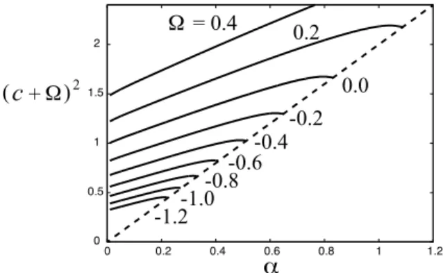
(4) 12 Figure 2 demonstrates peaking phenomenon of wave profiles. Namely, the wave crest becomes sharper with increase of the wave amplitude‐to‐depth ratio \alpha=a/h , and the limiting wave has a corner at the crest. It should be noted that, for \Omega<0 , the wave amplitude of the limiting wave decreases with increase of the absolute value |\Omega|. Figure 3 shows variation of the wave speed c with the wave amplitude‐to‐depth ratio \alpha=a/h . It is found that, for each value of \Omega , the wave speed c of the limiting wave attains a critical value which is shown by the dashed line in fig.3. This critical value can be analytically determined as follows. First, the boundary condition on the water surface y=\tilde{y}_{0}(x) is given by Bernoulli’s theorem as. U^{2}+V^{2}+2y=(c+\Omega)^{2}. on y=\tilde{y}_{0}(x). (6). Since the crest of the limiting wave is the stagnation point, namely U=V=0 at y=\alpha=a/h , we can get a critical condition among \alpha, c and \Omega for the limiting wave as. 2\alpha=(c+\Omega)^{2}. (7). The dashed line in fig.3 shows this condition.. (c+\Omega)^{2}. 0. 02. 04. 06. 08. 1. 12. \alpha. Fig.3. Variation of the wave speed c with the wave amplitude‐to‐depth ratio \alpha=a/h. Numerals in the figure show the value of the shear strength \Omega . The dashed line. denotes the critical condition (7). Solutions of the full Euler system are numerically obtained using the boundary integral method [17].. 2.3. Crest singularities of peaked waves. In this subsection, we consider singularities at the wave crest of peaked waves. For that,. the origin of the z ‐plane is set to the wave crest, as shown in figs.4(a) and (b). In the case of no shear current, namely \Omega=0 , Stokes [15, p.225] found that the inner angle of the corner at the crest of the peaked wave is 120 degrees from local flow analysis near. the wave crest, and Grant [7] showed existence of high‐order singularities using conformal mapping of the flow domain into the complex velocity potential f‐plane. For \Omega=0 , the f‐plane is suitable for local flow analysis near the wave crest, because the water surface.

(5) 13 is mapped onto the real axis \psi=0 . On the other hand, for \Omega\neq 0 , the water surface is not located on \psi=0 , as shown in fig.4(c), and thus it is necessary to introduce a new complex plane, the \zeta ‐plane (\zeta=\xi+i\eta) , as shown in fig.4(d), where the flow domain mapped onto the lower half plane (\eta<0) and the water surface is mapped onto the real axis \eta=0 . In the \zeta ‐plane, steady wave solutions are given by for z=z(\zeta) and f=f(\zeta) , and the kinematic and dynamic conditions for them on the water surface \eta=0 can be written, respectively, as. \psi_{\xi}+\Omega(1+\alpha+y)y_{\xi}=0. on. (8). \eta=0. and. \frac{1}{x_{\xi^{2} +y_{\xi^{2} }\{\phi_{\xi}+\Omega(1+\alpha+y)x_{\xi}\}^{2}+ 2(\alpha+y)=(c+\Omega)^{2}. on \eta=0. (9). ). (a) Local flow near the wave crest. (b) The. z=0. z. plane (z=x+iy). D)^{2}\}. (c) The f plane. Fig.4. (f=\phi+i\psi). (d) The \zeta plane (\zeta=\xi+i\eta). Conformal mapping of the flow domain for local flow analysis near the wave crest.. We may assume that the local solutions z(\zeta) and f(\zeta) near the wave crest \zeta=0 are represented by. z(\zeta) = \^{A}_{0}\zeta^{\hat{\mu}0}+\hat{A}_{1}\zeta^{\hat{\mu}_{1} + f(\zeta) = c\zeta+\hat{B}_{0}\zeta^{\hat{\nu}_{0}}+. ,. (|\zeta|\ll 1). (10).

(6) 14 where \hat{\mu}_{1}>\hat{\mu}_{0}>0 and \hat{\nu}_{0}>0 . Substituting these into the free surface conditions (8) and (9) and matching the leading order terms, we can determine the coefficients \hat{\mu}_{0}, \^{A}_{0} and \hat{B}_{0} in (10) as. \hat{\mu}_{0}=\hat{\nu}_{0}=\frac{2}{3} , \^{A}_{0}=(\frac{3}{2}c)^{2/3}e^{- i\pi/6} \hat{B}_{0}=-\Omega(1+\alpha)\^{A}_{0}. (11). This result indicates that the inner angle of the corner at the crest of the peaked waves is always 120 degrees, and does not depend on the shear strength \Omega . This agrees with the. previous result from another approach [11, §14.50]. It should be noted that the present method allows us to examine high‐order singularities even for \Omega\neq 0 , similarly to [7] for \Omega=0.. 3. Long wave models of solitary waves on a linear shear current. In this section, we introduce the two long wave models, the Korteweg‐de Vries (KdV) model and the strongly nonlinear model, which can produce peaking phenomenon, and investigate linear stability of steady solutions of these models. 3.1 3.1.1. The two long wave models The Korteweg‐de Vries (KdV) model [1, 4, 6]. For weakly nonlinear long waves (h/L=\epsilon\ll 1 and a/h=\alpha=O(\epsilon^{2}), L : a typical horizontal length scale), we can derive the Korteweg‐de Vries (KdV) model [1, 4, 6] which can be written in the frame of reference moving to the left with constant speed. \tilde{y}_{t}+(c-c_{0})\tilde{y}_{x}-c_{1}\tilde{y}\tilde{y}_{x}-c_{2}\tilde{y} _{xxx}=0. c. as. (12). where \tilde{y}=\tilde{y}(x, t) is the wave elevation,. c_{0}=- \frac{1}{2}\Omega+\sqrt{1+\frac{1}{4}\Omega^{2} , c_{1}= \frac{(c_{0}+\Omega)^{3}+2(c_{0}+\Omega)-\Omega}{1+(c_{0}+\Omega)^{2}. and. c_{2}= \frac{1}{3}\frac{(c_{0}+\Omega)^{3} {1+(c_{0}+\Omega)(13) ^{2}. A steady solution \tilde{y}_{0}(x) of (12) is given by. \tilde{y}_{0}(x)=\alpha sech2 k_{0}x. (14). with. c=c_{0}+ \frac{1}{3}c_{1}\alpha. and. k_{0}^{2}= \frac{1}{12}\frac{c_{1} {c_{2} \alpha. (15). Note that a steady solution \tilde{y}_{0}(x) in (14) decays exponentially as \tilde{y}_{0}(x)arrow 4\alpha e^{\mp 2k_{0}x} (xarrow\pm\infty) ..

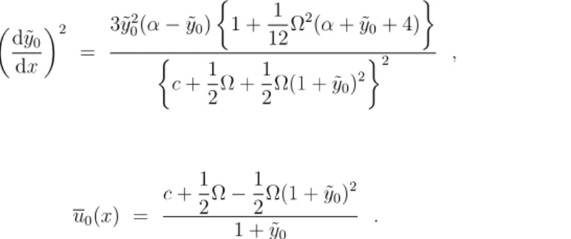
(7) 15 3.1.2. The strongly nonlinear model [4]. Choi [4] derived another class of long wave model for fully nonlinear and weakly dispersive waves, namely for long waves without assuming weak nonlinearity. This model is called the strongly nonlinear model and expressed as. \{begin{ar y}{l \tilde{y}_t+\Omega(1+\tilde{y})\tilde{y}_x+\partil_{x}\(1+\tilde{y}) \overlin{u}\=0 \overlin{u}_t+\overlin{u}\overlin{u}_x+\tilde{y}_x=\frac{1}3\frac{1} {1+\tilde{y}\partil_{x}[(1+\tilde{y})^2D_{t}\(1+\tilde{y})\overlin{u}_x \}] \end{ar y}. (16). where the depth mean horizontal velocity \overline{u}=\overline{u}(x, t) and the differential operator D_{t} are defined, respectively, by. \overline{u}(x, t)=\frac{1}{1+\tilde{y} \int_{-1}^{\tilde{y} u(x, y, t)dy. and. D_{t}=\partial_{t}+\{\overline{u}+\Omega(1+\tilde{y})\}\partial_{x}. (17). Note that, for \Omega=0, (16) corresponds to the Green‐Naghdi model [8]. Steady solutions \tilde{y}_{0}(x) and \overline{u}_{0}(x) of the strongly nonlinear model are given, respectively, by [1, 4]. and. (\frac{d\tile{y}_0{dx})^{2=\frac{3\tilde{y}_0^{2}(\alph-\tilde{y}_0) \{1+frac{1} 2\Omega^{2}(\alph+\tilde{y}_0+4)\}{ c+\frac{1}2\Omega+ \frac{1}2\Omega(1+\overlin{y}_0)^{2}\^{2} \overline{u}_{0}(x)=\frac{ +\frac{1}{2}\Omega-\frac{1}{2}\Omega(1+\tilde{y} _{0})^{2}{1+\tilde{y}_{0}. (18). (19). Here it should be remarked that the denominator of (18) vanishes at a critical value \Omega_{critica{\imath} of the shear strength. \Omega. given by. \Omega_{critica1}=\frac{12}{\alpha(3\alpha^{2}+9\alpha+8)}. (20). and that the wave slope at the crest |d\tilde{y}_{0}/dx|_{crest}arrow\infty as \Omegaarrow\Omega_{critica{\imath}} . This may be. related to peaking phenomenon. Also note that a steady solution \tilde{y}_{0}(x) in (14) decays exponentially as \tilde{y}_{0}(x)arrow ae^{\mp\kappa_{0}x}(xarrow\pm\infty) with the decay rate \kappa_{0} given by. \kap a_{0^{2} =3\frac{c(c+\Omega)-1}{(c+\Omega)^{2} 3.1.3. (21). Peaking phenomenon. Figure 5 compares some computed results of wave profiles of steady solutions of the two. long wave models, the. KdV. model (12) and the strongly nonlinear model (16), with. those of the full Euler system for different negative values of \Omega(-3.2\leq\Omega\leq-0.5) with the wave amplitude‐to‐depth ratio \alpha fixed to 0.05. Solutions of the full Euler system.

(8) 16 was numerically obtained using the boundary integral method [17]. It is found that both the long wave models captures peaking phenomenon qualitatively very well, and quantitatively the strongly nonlinear model is slightly more accurate than the KdV model.. y. y. y. (a). ( b). \Omega=-0.5. ( c). \Omega=-1.0. \Omega=-15. 0 D6. — Euler — SNL. 005. j. :I. : k:. .. KdV. 004 :\ovalbox{\tt\small REJECT} 1 :. y003. y. y. t:. :I. I:. :I. :I :t :I. 002. 1:. S: i:. :l S\backslash ^{:}. \backslash :. 0 OI. \near ow \backslash :\backslash _{\dot{Y} 0. x. (d). Fig.5. ( e). \Omega=-2.0. ( f). \Omega=-2.5. \Omega=-3.2. Comparison of wave profiles of steady solutions. The wave amplitude‐to‐depth ratio \alpha=a/h is fixed to 0.05.. Solid line: the full Euler system, dashed line: the strongly nonlinear model (SNL). and dotted line: the. KdV. model. Solutions of the full Euler system are. numerically obtained using the boundary integral method [17].. 3.2. Linear stability. 3.2.1. The. KdV. model [2, 9]. Substituting. \tilde{y}(x, t)=\tilde{y}_{0}(x)+\tilde{y}_{1}(x, t) into the. KdV. with \tilde{y}_{1}(x, t)arrow 0(xarrow\pm\infty). (22). model (12), linearizing it on the assumption of |\tilde{y}_{1}|\ll 1 and introducing. separation of variable. \tilde{y}_{1}(x, t)=e^{\sigma t}Y(x). (23). we get. c_{2}Y_{x x}+c_{1} \{\tilde{y}_{0}(x)-\frac{1}{3}\alpha\}Y_{x}+c_{1}\tilde{y} _{0x}Y=\sigma Y. for. -\infty<x<\infty. (24).

(9) 17 This equation for. -\infty<x<\infty. can be transformed using. with k_{0} defined by (15). z=\tanh k_{0}x. into the form of a Fuchian equation for. -1<z<1. (25). as. \tilde{Y}_{z z}+\frac{A_{2}(z)}{1-z^{2} \tilde{Y}_{z }+\frac{A_{1}(z)}{(1- z^{2})^{2} \tilde{Y}_{z}+\frac{A_{0}(z;\sigma)}{(1-z^{2})^{3} \tilde{Y}=0. for. -1<z<1. (26). \tilde{Y}(z)=Y(x(z)) , and A_{0}(z;\sigma), A_{1}(z) and A_{2}(z) are analytic in the neighborhood of [−1, 1]. Then we can apply Frobenius’ theory and represent \tilde{Y}(z) by. where. \tilde{Y}(z)= (\frac{1+z}{1-z})^{\mu}\sum_{n=0}^{\infty}a_{n}(1+z)^{n} where. \mu. (27). is a solution of the indicial equation. I(\mu, \sigma)=\mu^{3}-\mu+\sigma=0. (28). Note that \mu in (28) corresponds to the ratio \kappa_{1}/\kappa_{0} where \kappa_{1} denotes the exponential decay rate of the eigenfunction Y(x) in (24) as Y(x)arrow a\pm e^{\mp\kappa_{1}x}(xarrow\pm\infty) , and \kappa_{0}=2k_{0} is that of the steady solution \tilde{y}_{0}(x) in (14). Substituting (27) into (26), we get. \tilde{Y}(z)=z(1-z^{2}). or. Y(x)= sech2 k_{0}x\cdot\tanh k_{0}x. (29). and \sigma=0. Thus steady solutions (14) of the. 3.2.2. KdV. (30). model (12) are neutrally stable.. The strongly nonlinear model. For linear stability analysis of the strongly nonlinear model (16), it is convenient to. transform it to a conserved form as. \{ begin{ar ay}{l \tilde{y}_{t}+w_{x}=0 w_{t}+\partial_{x}G(\tilde{y},w)=0 \end{ar ay} where. w. and G=G(\tilde{y}, w) are defined, respectively, by. w=( \tilde{y}+1)\overline{u}+\frac{1}{2}\Omega(\tilde{y}+1)^{2} and. (31). (32).

(10) 18. G( \tilde{y}, w)=\frac{w^{2} {\tilde{y}+1}+\frac{1}{2}(\tilde{y}+1)+\frac{1} {12}\Omega^{2}(\tilde{y}+1)^{3}-\frac{1}{3}(\tilde{y}+1)^{2}D_{t}\{(\tilde{y}+1) \partial_{x}(\frac{w}{\tilde{y}+1}-\frac{1}{2}\Omega(\tilde(33) {y}+1) \} D_{t}=\partial_{t}+\{\frac{w}{\tilde{y}+1}+\frac{1}{2}\Omega(\tilde{y}+1)\} \partial_{x} which is constant. Note that, for with. . The steady solution of. \Omega=0 ,. w. is given by. w_{0}=c+ \frac{1}{2}\Omega. Li [10] examined linear stability of steady. solutions of the strongly nonlinear model using this conserved form. Substituting. \tilde{y}(x)=\tilde{y}_{0}(x)+\tilde{y}_{1}(x, t). and. w(x)=w_{0}+w_{1}(x, t). (34). into (31), linearizing them on the assumption of |\tilde{y}_{1}|, |w_{1}|\ll 1 , and introducing separation of variables. \tilde{y}_{1}(x, t)=e^{\sigma t}Y(x). and. w_{1}(x, t)=e^{\sigma t}W(x). (35). we get. \{ begin{ar y}{l \sigmaY+W_{x}=0 \sigmaW+\frac{\partial}{\partialx}\{ sigma(\mathcal{P}_{1}W+\mathcal{P}_{2}Y)- (\mathcal{P}_{3}W+\mathcal{P}_{4}Y)\}=0 \end{ar y}. (36). where \mathcal{P}_{j} ’s are linear operators. In addition, introducing a new variable Q(x) defined by. Q(x)= \int_{-\infty}^{x}Wdx. (37). \{ begin{ar ay}{l \sigmaY+Q_{x }=0 \sigma(Q+\mathcal{P}_{1}Q_{x}+\mathcal{P}_{2}Y)-(\mathcal{P}_{3}Q_{x}+ \mathcal{P}_{4}Y)=0 \end{ar ay}. (38). we can rewrite (36) as. This can be summarized in the form of a generalized eigenvalue problem as. \mathcal{L}(Y, Q)=\sigma \mathcal{R}(Y, Q). (39). where \mathcal{L} and \mathcal{R} are linear operators. Note that the eigenfunction Y(x) decays exponen‐ tially as Y(x)arrow a\pm e^{\mp\kappa_{1}x}(xarrow\pm\infty) with the decay rate \kappa_{1} satisfying. (1- \frac{1}{3}\kap a_{1^{2} )(\kap a_{1}\mp\sigma)^{2}-\frac{\Omega}{c+\Omega} \kap a_{1}(\kap a_{1}\mp\sigma)-\frac{1}{(c+\Omega)^{2} \kap a_{1^{2} =0. (40). Using finite difference approximation, we may numerically solve (39). However the. infinite range -\infty<x<\infty of the domain of Y and Q caused some numerical troubles to get accurate solutions. One of remedies for these troubles may be change of variable.

(11) 19 such as (25) for the KdV model. In the case of the strongly nonlinear model, similarly to (25), we can introduce z=\tanh k_{0}x. where. \kappa_{0}. with k_{0}=\kappa_{0}/2. (41). is the exponential decay rate of the steady solution \tilde{y}_{0}(x) and given by (21). Then. -\infty<x<\infty. is transformed to. -1<z<1 ,. and \tilde{Q}(z)=Q(x(z)) have singularities at. and the eigenfunctions. z=\pm 1. \tilde{Y}(z)=Y(x(z)). such as (27) in the case of the. model. These singularities can be regularized using the exponential decay rate. \kappa_{1}. KdV. of the. eigenfunction Y(x) in (40), similarly to (27). It should be noted that Camassa & Wu [3] applied the similar numerical method to linear stability analysis of steady solutions of the forced KdV model.. 4. Conclusions. We have considered two‐dimensional steady motion of solitary waves progressing in per‐ manent form with constant speed on a shear current of which the horizontal velocity varies linearly with depth, as shown in fig. 1. In particular, peaking phenomenon, namely peaking of wave profiles with increase of amplitude as shown in fig.2, has been studied. First, crest singularities of the peaked wave were investigated using local flow analysis near the wave crest with conformal mapping in fig.4. It was shown that the inner angle of the corner at the crest of the peaked wave does not depend on the magnitude of shear current. It should be noted that this method of local flow analysis enables us to examine high‐order singularities. Next, for systematic understanding peaking phenomenon, the two long wave models,. the Korteweg‐de Vries (KdV) model (12) and the strongly nonlinear model (16), were introduced. Numerical comparison of steady solutions of these models with those of the full Euler system demonstrated that these long wave models can qualitatively capture variation of peaking phenomenon with the shear strength \Omega , as shown in fig.5. In addition, linear stability analysis of steady solutions of these long wave models was discussed. Similarly to the case of solitary waves without shear current (\Omega=0) , we can. analytically show that steady solutions of the. KdV. model (12) are neutrally stable for all. \Omega\neq 0 . On the other hand, linear stability analysis of steady solutions of the strongly. nonlinear model (16) requires numerical computation with suitable change of variable and representation of eigenfunctions such as (41) and (27), respectively. This and its application to the full Euler system remain as future works.. Acknowledgments This work was supported in part by JSPS KAKENHI Grant No. JP17H02856.. References. [1] Benjamin, T.B. : The solitary wave on a stream with an arbitrary distribution of vorticity, J. Fluid Mech., vol.12, pp.97‐116, 1962..

(12) 20 [2] Berryman, J.G. : Stability of solitary waves in shallow water, Phys. Fluids, vol.19, pp.771‐777, 1976.. [3] Camassa, R. and Wu, T.Y. : Stability of forced steady solitary waves, Phil. Trans. R. Soc. Lond. A, vo1.337, pp.429‐466, 1991.. [4] Choi, W. : Strongly nonlinear long gravity waves in uniform shear flows, Physical Review E, vo1.68, 026305, 2003.. [5] Francius, M. and Kharif, C. : Two‐dimensional stability of finite‐amplitude gravity waves on water of finite depth with constant vorticity, J. Fluid Mech., vol.830, pp.631‐659, 2017.. [6] Freeman, N.C. and Johnson, R.S. : Shallow water waves on shear flows, J. Fluid Mech., vol.42, pp.401‐409, 1970.. [7] Grant, M.A. : The singularity at the crest of a finite amplitude progressive Stokes wave, J. Fluid Mech., vol.59, pp.257‐262, 1973.. [8] Green, A.E. and Naghdi, P.M. : A derivation of equations for wave propagation in water of variable depth, J. Fluid Mech., vol.78, pp.237‐246, 1973.. [9] Jeffery, A. and Kakutani, T. : Stability of the Burgers shock wave and the Korteweg‐ de Vries soliton, Indiana University Mathematics Journal, vol.20, pp.463‐468, 1970.. [10] Li, Y.A. : Linear stability of solitary waves of the Green‐Naghdi equations, Com‐ munications on Pure and Applied Mathematics, vol.54, pp.501‐536, 2001.. [11] Milne‐Thomson, L.M. : Theoretical hydrodynamics, 5th ed., §14.50, Dover, 1968. [12] Okamura, M. and Oikawa, M. : The linear stability of finite amplitude surface waves on a linear shearing flow, J. Phys. Soc. Japan, vol.58, pp.2386‐2396, 1989.. [13] Peregrine, D.H. : Interaction of water waves and currents, Adv. Appl. Mech., vol.16, pp.9‐117, 1976.. [14] Pullin, D.I. and Grimshaw, R.H.J. : Finite‐amplitude solitary waves at the interface between two homogeneous fluids, Phys. Fluids, vol.31, pp.3550‐3559, 1988.. [15] Stokes, G.G. : On the theory of oscillatory waves. Appendix B., Math. and Phys. Pap., vol.1, pp.197‐229, pp.314‐326, 1880.. [16] Teles da Silva, A.F. and Peregrine, D.H. : Steep, steady surface waves on water of finite depth with constant vorticity, J. Fluid Mech., vol.195, pp.281‐302, 1988.. [17] Vanden‐Broeck, J.‐M. : Steep solitary waves in water of finite depth with constant vorticity, J. Fluid Mech., vol.274, pp.339‐348, 1994..

(13)