Robust Adaptive Output Feedback Control of MIMO Systems Using Multirate Sampling

Robust Adaptive Output Feedback Control of MIMO Systems Using Multirate Sampling

Ikuro Mizumoto* Satoshi Ohdaira Makoto Kumon and Zenta Iwai Department of Mechanical System Engineering

Kumamoto University

2-39-1 Kurokami, Kumamoto, 860-8555, Japan

*

[email protected] Abstract

— In adaptive output feedback control based on al-

most strictly positive real (ASPR) conditions, a technical difficulty arises when the controlled multi-input multi-output (MIMO) system is non-square. To overcome this, the idea of multirate sampled-data control has been proposed. That is, through careful choice of faster input sampling rates create a lifted discrete- time system which has the same number of inputs and outputs and does not give rise to the causality constraint. The output feedback based adaptive control strategy can then be applied to this lifted system under certain conditions. In this report, we propose a robust adaptive controller design scheme for non- square MIMO systems using the multirate sampling strategy without the causality problem.

Keywords—adaptive

output feedback control, multirate sampled-data control, MIMO systems, almost strictly positive real

I. I

NTRODUCTION

Adaptive output feedback control design based on almost strictly positive real (ASPR) conditions has several practical advantages and has been applied successfully to many in- dustrial processes. The design procedure for such adaptive control scheme, however, requires a technical assumption that the systems to be controlled must be square, i.e., the number of inputs must be equal to the number of outputs [1], [2], [3], [4], [5]. Although this requirement is automatically satisfied to SISO plants [6], [7], [8], it can be quite restrictive because in many practical MIMO systems, the number of inputs is less than that of the outputs, especially in cases where several control objectives are to be achieved. As a countermeasure to this problem, the application of digital control with a multirate sampling scheme has been considered on purpose in order to obtain a multirate system with square structure so as to accommodate existing adaptive control strategies [9]. By carefully selecting different sampling rates, the method ensures that the resultant systems after lifting [10], [11] are square (with the same number of inputs and outputs) without causality constraint.

In this paper, we present a robust adaptive controller design scheme for non-square MIMO systems using the multirate sampling strategy. Considering the ASPR based adaptive out- put feedback control of discrete time systems, the controlled system should be proper so that the causality problem in the controller appears in general. We propose a design scheme of robust adaptive control which can solve the causality problem

- Hmr - G

_c

- S

_T

-

u u

_c

y

_c

y

Fig. 1. The multirate sampled-data system

and show that all the signals in the closed loop system are bounded.

II. M

ULTIRATE

S

AMPLING AND

L

IFTING

Consider a continuous-time, linear, time-invariant plant G

_c

with m inputs and p outputs.

˙

x

_c

(t) = A

_c

x

_c

(t) + B

_c

u

_c

(t) + η

_c

(t), (1)

y

_c

(t) = Cx

_c

(t), (2)

where x

_c

∈ R

ⁿ

is a state vector, y

_c

∈ R

^p

and u

_c

∈ R

^m

are output and input vectors, respectively, and η

_c

is a disturbance.

We assume that p > m and B

_c

is partitioned according to the input u

_c

as follows:

B

_c

= [b

_c1

b

_c2

· · · b

_cm

], u

_c

= [u

_c1

, u

_c2

, · · · , u

_cm

]

^T

, in which b

_ci

, i = 1, · · · , m are n-dimensional column vectors.

The system G

_c

is a typical non-square system so that one can not directly apply the ASPR based adaptive output feedback strategy. To overcome this problem, the use of multi- rate sampling and lifting techniques has been presented [9] in order to derive a square lifted discrete time system.

Consider choosing all outputs uniformly with a single period, say, T, and update the inputs u

_c1

, u

_c2

, · · · , u

_cm

through zero-order holds with fast periods T /q

₁

, T /q

₂

, · · · , T /q

_m

, respectively. Here q

₁

, q

₂

, · · · , q

_m

are all positive integers and are chosen to satisfy

q

₁

+ q

₂

+ · · · + q

_m

= p. (3) We remark that such q

_i

’s always exist (if m < p) and are non-unique; e.g., if m = 2 and p = 5, there are four possible (q

₁

, q

₂

) pairs satisfying (3); they are (1, 4), (2, 3), (3, 2), and (4, 1).

Denoting the correspondingly discretized system by G, the obtained multirate discrete-time system depicted in Figure 1 can be expressed by

G = S

_T

G

_c

Hmr ,

where S

_T

is an ideal sampler with period T (vector-valued), and Hmr is the multirate zero-order hold operator defined as

Hmr = diag[H

_{T /qi}

]

_i=1,···,m

with H

_{T /qi}

being the synchronized zero-order hold with period T /q

_i

. Note that y is single-rate with period T (y = S

_T

y

_c

), but u is multirate with each component having a different period;

we can write u =



  u

₁

.. . u

_m



  , u

_ci

= H

_{T /qi}

u

_i

, i = 1, 2, · · · , m.

Next, consider lifting this multirate system to arrive at a time-invariant one with the single period T .

Let v be a discrete-time signal defined on the time set { 0, 1, 2, · · ·} :

v = { v(0), v(1), v(2), · · ·} .

and consider the q-fold lifting operator L

_q

which maps v into v as follows [10], [11]:

v =

 

 



 

 



 

  v(0) v(1) .. . v(q − 1)



 

  ,



 

 

v(q) v(q + 1)

.. . v(2q − 1)



 

  , · · · ,

 

 



 

  .

The inverse lifting operation, L

⁻¹_q

is also defined obviously.

In order to get a lifted system which is single-rate with period T, we lift the input u

_i

by L

_qi

to get u

_i

. The lifted input u(k) is given by

u(k) =



  u

₁

(k)

.. . u

_m

(k)



  .

Thus the lifted system G which maps u(k) into y(k) can be expressed as:

G = G



  L

⁻¹_q

1

. ..

L

⁻¹_q

m



 

This G is the m × m square system, based on (3) and is time- invariant. The state-space model of G can be derived based on the results in [12], [13] as follows:

x(k + 1) = Ax(k) + Bu(k) + η

_d

(k), (4)

y(k) = Cx(k), (5)

where

A = e

^AcT

, B =

B

₁

B

₂

· · · B

_m

C = C

_c

, B

_i

=

A

^q_iⁱ⁻¹

B

_i

· · · A

_i

B

_i

B

_i

A

_i

= e

^{AcT /qi}

, b

_i

=

_{T /qi}

0

e

^Act

B

_ci

dt, i = 1, 2, · · · , m.

η

_d

(k) =

_(k+1)T

kT

e

^{Ac{(k+1)T−τ}}

η

_c

(τ) dτ

Due to the choice of sampling rates, the causality constraint in the lifted controller (mapping y into u) will not arise [12].

III. A

DAPTIVE

C

ONTROL

D

ESIGN

The robust adaptive controller is designed for the lifted square system G in (4) and (5).

A. Problem Statement

Consider the lifted, but square system G in (4) and (5);

We shall recall a few definition concerning the ASPR-ness of discrete systems in order to proceed.

Definition 1: (Almost Strictly Positive Realness [2], [5]) The square plant G in (4) and (5) is called almost strictly positive real (ASPR) if there exists a static output feedback such that the resulting closed loop system is strictly positive real (SPR). Explicitly, G is ASPR if there exists a control input with a feedback gain Θ

^∗

,

u(k) = − Θ

^∗

y(k) + v(k), (6) (v is any external input) such that the resulting closed loop system from v(k) to y(k),

x(k + 1) = A

_cl

x(k) + B

_cl

v(k), (7) y(k) = C

_cl

x(k) + D

_cl

v(k), (8) with

A

_cl

= A − BΘ

^∗

(I + DΘ

^∗

)

⁻¹

C, B

_cl

= B(I + Θ

^∗

D)

⁻¹

, C

_cl

= (I + DΘ

^∗

)

⁻¹

C , D

_cl

= D(I + Θ

^∗

D)

⁻¹

,

(9) is SPR.

Definition 2: (Strong ASPR-ness [9]) The square plant G is called strongly ASPR if there exists a static output feedback,

u(k) = − Θ

^∗

y(k) + v(k),

such that the closed loop system with state matrices (A

_cl

, B

_cl

, C

_cl

, D

_cl

) as given in (9) is SPR and, in addition, a transformed closed loop system with ˜ v = (I + Θ

^∗

D)

⁻¹

v as input,

x(k + 1) = A

_cl

x(k) + B˜ v(k) (10) y(k) = C

_cl

x(k) + D v(k) ˜ (11) is also SPR.

The sufficient conditions for G to be ASPR are easily obtained by translating the conditions given for continuous- time systems [14] as follows.

ASPR Conditions:

(1) The relative MacMillan degree of the system is n/n, where n is the dimension of the A-matrix.

(2) The plant is minimum-phase.

Furthermore, for strong almost strictly positive realness, an additional condition is required [9]:

(3) D + D

^T

> 0.

We shall impose the following assumptions on the lifted model G in (4) and (5).

Assumption 1: The plant G given in (4) and (5) is control-

lable and observable.

This assumption can be related to controllability and ob- servability of the original continuous-time system and a non- pathological sampling condition [13], [12].

Assumption 2: For the plant G given in (4) and (5) with η

_d

(k) ≡ 0, there exists a known static feedforward compen- sator (PFC) D such that the resulting augmented system with a state-space model,

x(k + 1) = Ax(k) + Bu(k), (12) y

_a

(k) = y(k) + Du(k) = Cx(k) + Du(k), (13) is strongly ASPR.

Assumption 3: The disturbance η

_d

(k) can be represented as

η

_d

(k) = Bη(k) (14)

Assumption 4: Denoting η(k) = [η

₁

, · · · , η

_m

], there exist positive constant β

_i^∗

such that

| η

_i

(k) | ≤ β

_i^∗

(15) It should be noted that under Assumption 2, there exists a static output feedback with a feedback gain matrix Θ ˜

^∗_e

> 0,

u(k) = − Θ ˜

^∗_e

y

_a

(k) + v(k)

such that the resulting closed loop system, after an input transformation ˜ v = (I + ˜ Θ

^∗_e

D)

⁻¹

v,

x(k + 1) = A

_ac

x(k) + B˜ v(k), y

_a

(k) = C

_ac

x(k) + D˜ v(k),

is SPR. Where

A

_ac

= A − B Θ ˜

^∗_e

(I + D Θ ˜

^∗_e

)

⁻¹

C, C

_ac

= (I + D Θ ˜

^∗_e

)

⁻¹

C.

Further, since the system (A

_ac

, B, C

_ac

, D) is SPR, there exist positive symmetric matrices P = P

^T

> 0, Q = Q

^T

> 0 and appropriate matrices L and W such that based on the Kalman- Yakubovich Lemma, the following hold:

A

^T_ac

P A

_ac

− P = − LL

^T

− Q, A

^T_ac

P B = C

_ac^T

− LW

^T

,

B

^T

P B = D + D

^T

− W W

^T

.

(16) Our objective in this paper is to design a robust adaptive controller that ensures the boundedness of all signals in the control system for G with disturbances under Assumptions 1 to 4.

B. Controller Design Procedure

The robust adaptive controller is designed as follows:

u(k) = u

_e

(k) + u

_r

(k) (17)

u

_e

(k) = − Θ

_e

(k)y(k) (18)

u

_ri

(k) = − β

_i

(k)sgn (y

_ai

(k)) , i = 1, 2, · · · , p (19) where u

_ri

(k) is the i-th element of u

_r

(k) and y

_ai

(k) is the i-th element of y

_a

(k), i.e.

u

_r

(k) = [u

_r1

(k) · · · u

_rp

(k)]

^T

,

y

_a

(k) = [y

_a1

(k) · · · y

_ap

(k)]

^T

(20)

The feedback gain matrix Θ

_e

(k) in (18) is adaptively adjusted by the following parameter adjusting law:

Θ

_e

(k) = Θ

_Ie

(k)+Θ

_{P e}

(k) (21) Θ

_Ie

(k) = Θ

_Ie

(k − 1)+y

_a

(k)y(k)

^T

Γ

_Ie

− σΘ

_Ie

(k) (22) Θ

_{P e}

(k) = y

_a

(k)y(k)

^T

Γ

_{P e}

(23) with Γ

_Ie

= Γ

^T_Ie

> 0, Γ

_{P e}

= Γ

^T_{P e}

> 0 and σ > 0. The gains in the robust adaptive controller (19) are adjusted by the following parameter adjusting law:

β

_i

(k) = β

_Ii

(k) + β

_{P i}

(k) (24) β

_Ii

(k) = β

_Ii

(k − 1)sgn (y

_ai

(k))

+γ

_βIi

| y

_ai

(k) | − σ

_βi

β

_Ii

(k) (25) β

_{P i}

(k) = γ

_{βP i}

| y

_ai

(k) | (26) with γ

_βIi

> 0, γ

_{βP i}

> 0 and σ

_βi

> 0. The parameter adjusting laws (22) and (25) can be rewritten by

Θ

_Ie

(k) = ¯ σΘ

_Ie

(k − 1) + ¯ σy

_a

(k)y(k)

^T

Γ

_Ie

(27) β

_Ii

(k) = ¯ σ

_βi

β

_Ii

(k − 1)sgn (y

_ai

(k))

+¯ σ

_βi

γ

_βIi

| y

_ai

(k) | (28) with 0 < ¯ σ =

_1+σ¹

< 1 and 0 < ¯ σ

_βi

=

_1+σ¹

betai

< 1.

It is noted that y

_a

(k) in (19), (21) and (24) cannot be directly obtained from measured signals because of a causality problem arising from the direct feedthrough term D in (13).

However, y

_a

(k) can be generated by using available signals from (13) and (17) to (28) without the causality problem as follows:

y

_a

(k) =

I + Dy(k)

^T

Γ

_e

y(k) + DΓ

_β

₋₁

× (y(k) − σDΘ ¯

_Ie

(k − 1)y(k) − Db(k − 1)) (29) where

Γ

_Ie

= Γ

^T_Ie

> 0, Γ

_{P e}

= Γ

^T_{P e}

> 0, γ

_βIi

> 0, γ

_{βP i}

> 0 Γ

_e

= ¯ σΓ

_Ie

+ Γ

_{P e}

, Γ

_β

= diag

γ

_β1

, γ

_β2

, · · · , γ

_βp

γ

_βi

= ¯ σ

_βi

γ

_βIi

+ γ

_{βP i}

, i = 1, 2, · · · , p

b(k − 1) =



 

 

¯

σ

_β1

β

_I1

(k − 1)

¯

σ

_β2

β

_I2

(k − 1) .. .

¯

σ

_βp

β

_Ip

(k − 1)



 

 

C. Stability Analysis

Consider the following ideal control input:

u

^∗

(k) = u

^∗_e

(k) + u

^∗_r

(k) (30)

u

^∗_e

(k) = − Θ

^∗_e

y(k), (31)

Θ

^∗_e

=

I + ˜ Θ

^∗_e

D

₋₁

Θ ˜

^∗_e

= ˜ Θ

^∗_e

I + D Θ ˜

^∗_e

₋₁

(32)

u

^∗_r

(k) = −



 

 

β

^∗₁

sgn (y

_a1

(k)) β

^∗₂

sgn (y

_a2

(k))

.. . β

₂^∗

sgn (y

_ap

(k))



 

  (33)

The closed loop system with control input in (17) can be represented by

x(k + 1) = ˜ Ax(k) + B∆u(k) (34) y

_a

(k) = ˜ Cx(k) + D∆u(k) − Dη(k) (35) where

A ˜ = A − BΘ

^∗_e

C, C ˜ = (I − DΘ

^∗_e

)C (36)

∆u(k) = ∆u

_e

(k) + ∆u

_r

(k) + η(k) + u

^∗_r

(k) (37)

∆u

_e

(k) = u

_e

(k) − u

^∗_e

(k) = − ∆Θ

_e

(k)y(k) (38)

∆Θ

_e

(k) = Θ

_e

(k) − Θ

^∗_e

. (39)

∆u

_r

(k) = u

_r

(k) − u

^∗_r

(k) (40) Since it follows from (32) that

I − DΘ

^∗_e

= I − D Θ ˜

^∗_e

(I + D Θ ˜

^∗_e

)

⁻¹

= (I + D

_a

Θ ˜

^∗_e

)

⁻¹

= 0 (41) we have from (36) and (32) that

A ˜ = A − B Θ ˜

^∗_e

(I + D Θ ˜

^∗_e

)

⁻¹

C = A

_ac

, (42) C ˜ = (I + D Θ ˜

^∗_e

)

⁻¹

C = C

_ac

, (43) Thus, since the system (A

_ac

, B, C

_ac

, D) is SPR, there exist positive symmetric matrices P = P

^T

> 0, Q = Q

^T

> 0 such that the Kalman-Yakubovich Lemma in (16) is satisfied.

Now, consider the following positive definite function V (k), V (k) = V

₁

(k) + V

₂

(k) + V

₃

(k) (44)

V

₁

(k) = x

^T

(k)P x(k) (45)

V

₂

(k) = tr

¯

σ∆Θ

_Ie

(k − 1)Γ

⁻¹_Ie

∆Θ

_Ie

(k − 1)

^T

(46) V

₃

(k) =

p i=1

¯ σ

_βi

γ

_β⁻¹

Ii

∆β

_Ii²

(k − 1) (47)

where

∆Θ

_Ie

(k) = Θ

_Ie

(k) − Θ

^∗_e

, ∆β

_Ii

(k) = β

_Ii

(k) − β

_i^∗

(48) Define ∆V (k) by

∆V (k) = V (k + 1) − V (k) =

3 i=1

∆V

_i

(k) (49)

∆V

_i

(k) = V

_i

(k + 1) − V

_i

(k), i = 1, 2, 3 (50) First, we consider the difference ∆V

₁

. We have from (34), (45) and Kalman-Yakubovich Lemma in (16) that

∆V

₁

(k) ≤ − λ

_min

[Q] x(k)

²

− x(k)

^T

L + ∆u(k)

^T

W

²

+2y

^T_a

(k)∆u(k) + 2η

^T

(k)D

^T

∆u(k) (51) Next, consider the difference ∆V

₂

. From (27) and (48), we have

∆Θ

_Ie

(k − 1) = ¯ σ

⁻¹

∆Θ

_Ie

(k) − y

_a

(k)y(k)

^T

Γ

_Ie

(52) Thus ∆V

₂

(k) can be expressed as

∆V

₂

(k) = −

¯

σ

⁻¹

− ¯ σ tr

∆Θ

_Ie

(k)Γ

⁻¹_Ie

∆Θ

_Ie

(k)

^T

+2tr

∆Θ

_Ie

(k)y(k)y

_a

(k)

^T

− ¯ σtr

y

_a

(k)y(k)

^T

Γ

_Ie

y(k)y

_a

(k)

^T

(53)

Since

∆Θ

_Ie

(k) = ∆Θ

_e

(k) − y

_a

(k)y(k)

^T

Γ

_{P e}

(54)

∆Θ

_e

(k) = Θ

_e

(k) − Θ

^∗_e

(55)

∆Θ

_e

(k)y(k) = − ∆u

_e

(k) (56) it follows that

∆V

₂

(k) ≤ −

¯

σ

⁻¹

− σ ¯ λ

_min

Γ

⁻¹_Ie

∆Θ

_Ie

(k)

²

− λ

_min

[¯ σΓ

_Ie

+ Γ

_{P e}

] y

_a

(k)

²

y(k)

²

− y

_a

(k)

²

y(k)

^T

Γ

_{P e}

y(k) − 2y

_a

(k)

^T

∆u

_e

(k) (57) Next, consider the difference ∆V

₃

. From (28) and (48), we have

∆β

_Ii

(k − 1) = ¯ σ

_β⁻¹

i

∆β

_Ii

(k)sgn (y

_ai

(k)) − γ

_βIi

y

_ai

(k) (58) Thus ∆V

₃

(k) can be expressed as

∆V

₃

(k) = −

p i=1

(¯ σ

⁻¹_β

i

− σ ¯

_βi

)γ

⁻¹_β

Ii

∆β

_Ii

(k)

²

−

p i=1

¯

σ

_βi

γ

_βIi

y

_ai

(k)

²

+2

p

i=1

∆β

_Ii

(k)sgn (y

_ai

(k)) y

_ai

(k). (59) Further, since

∆β

_Ii

(k) = ∆β

_i

(k) − γ

_{βP i}

| y

_ai

(k) | (60)

∆β

_i

(k) = β

_i

(k) − β

_i^∗

(61)

∆β

_i

(k)sgn (y

_ai

(k)) y

_ai

(k) = − ∆u

_ri

(k)y

_ai

(k) (62)

∆V

₃

(k) can be evaluated by

∆V

₃

(k) = −

p i=1

¯ σ

_β⁻¹

i

− σ ¯

_βi

γ

⁻¹_β

Ii

| ∆β

_Ii

(k) |

²

−

p i=1

(¯ σ

_βi

γ

_βIi

+ γ

_{βP i}

) | y

_ai

(k) |

²

−

p i=1

γ

_{βP i}

| y

_ai

(k) |

²

− 2

p i=1

∆u

_ri

(k)y

_ai

(k) (63) Finally, from (51), (57)and (63), we have

∆V (k) ≤ − λ

_min

[Q] x(k)

²

− x(k)

^T

L + ∆u(k)

^T

W

²

−

¯

σ

⁻¹

− σ ¯ λ

_min

Γ

⁻¹_Ie

∆Θ

_Ie

(k)

²

− λ

_min

[Γ

_e

] y

_a

(k)

²

y(k)

²

− y

_a

(k)

²

y(k)

^T

Γ

_{P e}

y(k)

−

p i=1

¯ σ

⁻¹_β

i

− ¯ σ

_βi

γ

_β⁻¹

Ii

| ∆β

_Ii

(k) |

²

−

p i=1

γ

_βi

| y

_ai

(k) |

²

−

p i=1

γ

_{βP i}

| y

_ai

(k) |

²

+2η(k)

^T

D

^T

(∆u

_e

(k)+∆u

_r

(k)+η(k) + u

^∗_r

(k))

+2y

_a

(k)

^T

(η(k) + u

^∗_r

(k)) (64)

Here, we have

2y

_a

(k)

^T

(η(k) + u

^∗_r

(k))

≤ 2

p

i=1

{| y

_ai

(k) | β

_i^∗

+ | y

_ai

(k) | ( − β

_i^∗

) }

= 0 (65)

2η(k)

^T

D

^T

η(k) ≤ 2β

^∗2

D (66) 2η(k)

^T

D

^T

u

^∗_r

(k) ≤ 2β

^∗2

D (67) 2η(k)

^T

D

^T

∆u

_e

(k) ≤ 2β

^∗

D C ∆Θ

_Ie

(k) x(k)

+2β

^∗

D y

_a

(k) y

^T

(k)Γ

_{P e}

y(k) (68) with β

^∗

=

β

₁^∗2

+ β

^∗2₂

+ · · · + β

^∗2_p

_1/2

and 2η(k)

^T

D

^T

∆u

_r

(k)

≤ 2

p i=1

 



p j=1

β

_j^∗

| d

_ij

|

| ∆β

_Ii

(k) |

 

 +2

p i=1

 



p j=1

β

_j^∗

| d

_ij

|

γ

_{βP i}

| y

_ai

(k) |

 

 (69) where D = [d

_ij

] , i, j = 1, · · · , p. Further we have

− y

_a

(k)

²

y(k)

^T

Γ

_{P e}

y(k) + 2β

^∗

D y

_a

(k) y(k)

^T

Γ

_{P e}

y(k)

≤ − λ

_min

[Γ

_{P e}

] ( y

_a

(k) − β

^∗

D )

²

y(k)

²

+λ

_max

[Γ

_{P e}

] (β

^∗

)

²

C

²

D

²

x(k)

²

(70)

−

p

i=1

γ

_{βP i}

| y

_ai

(k) |

²

+ 2

p i=1

 



p j=1

β

_j^∗

| d

_ij

|

γ

_{βP i}

| y

_ai

(k) |

 



= −

p i=1

γ

_{βP i}

 

 | y

_ai

(k) | −





^p

j=1

β

_j^∗

| d

_ij

|





 



2

+

p i=1

γ

_{βP i}





^p

j=1

β

_j^∗

| d

_ij

|





2

(71) and it follows for any positive constants δ

₁

and δ

₂

that

− δ

₁

x(k)

²

+ 2β

^∗

D C ∆Θ

_Ie

(k) x(k)

= − δ

₁

x(k) − β

^∗

1

δ

₁

D C ∆Θ

_Ie

(k)

₂

+ (β

^∗

)

²

1

δ

₁

D

²

C

²

∆Θ

_Ie

(k)

²

(72)

− δ

₂

p i=1

∆β

_Ii²

(k) + 2

p i=1

 



p j=1

β

^∗_j

| d

_ij

|

| ∆β

_Ii

(k) |

 



= − δ

₂

p

i=1

 

 | ∆β

_Ii

(k) | − 1 δ

₂





^p

j=1

β

_j^∗

| d

_ij

|





 



2

+ 1 δ

₂

p i=1





^p

j=1

β

_j^∗

| d

_ij

|





2

. (73)

Thus ∆V (k) can finally be evaluated as

∆V (k)

≤ −

λ

_min

[Q]

− λ

_max

[Γ

_{P e}

] (β

^∗

)

²

C

²

D

²

− δ

₁

x(k)

²

−

¯

σ

⁻¹

− σ ¯ λ

_min

Γ

⁻¹_Ie

− (β

^∗

)

²

δ

₁

D

²

C

²

∆Θ

_Ie

(k)

²

−

p i=1

¯ σ

_β⁻¹

i

− σ ¯

_βi

γ

_β⁻¹

Ii

− δ

₂

| ∆β

_Ii

(k) |

²

+4 (β

^∗

)

²

D + 1 δ

₂

p i=1





^p

j=1

β

_j^∗

| d

_ij

|





2

+

p i=1

γ

_{βP i}





^p

j=1

β

^∗_j

| d

_ij

|





2

(74) Here, suppose that δ

₁

is chosen such that

(β

^∗

)

²

C

²

D

²

(¯ σ

⁻¹

− ¯ σ) λ

_min

Γ

⁻¹_Ie

< δ

₁

< λ

_min

[Q] − λ

_max

[Γ

_{P e}

] (β

^∗

)

²

C

²

D

²

(75) is satisfied. That is, σ, ¯ Γ

_Ie

and Γ

_{P e}

are designed such that there exists a δ

₁

which satisfies (75). Further suppose that δ

₂

is chosen such that

0 < δ

₂

<

p i=1

¯ σ

_β⁻¹

i

− σ ¯

_βi

γ

_β⁻¹

Ii

p . (76)

With δ

₁

and δ

₂

satisfying (75) and (76), the difference ∆V (k) can be evaluated as

∆V (k) ≤ − αV (k) + R (77)

R = 4 (β

^∗

)

²

D + 1 δ

₂

p i=1





^p

j=1

β

_j^∗

| d

_ij

|





2

+

p i=1

γ

_{βP i}





^p

j=1

β

^∗_j

| d

_ij

|





2

(78)

α = min





λ

_min

[Q] − λ

_max

[Γ

_{P e}

] (β

^∗

)

²

C

²

D

²

− δ

₁

λ

_max

[P ] ,

¯ σ

⁻¹

− σ ¯ λ

_min

Γ

⁻¹_Ie

− (β

^∗

)

²

δ

₁

D

²

C

²

!

λ

_max

Γ

⁻¹_Ie

,

2 i=1

¯ σ

⁻¹_β

i

− σ ¯

_βi

γ

⁻¹_β

Ii

− δ

₂

p i=1

γ

_β⁻¹

Ii



 

 

 (79)

y M

I m, u

L

φ c1

c2

g

Fig. 2. Cart-crane system

Table 1 Parameters of cart-crane system

Parameter Value

g 9.81 [m/s

²

]

M

(mass of the cart)

1.168 + 3 [kg]

m

(mass of the crane)

0.071 [kg]

L

(length to the center of gravity)

0.358 [m]

I

(moment of inertia)

3.025 × 10

⁻³

[kg · m

²

] c

₁

(damping constant of crane) 0.01 [N · s/rad]

c

₂

(damping constant of cart) 10 [N · s/m]

Consequently we have the following theorem concerning the boundedness of all the signals in the control system.

Theorem 1: Under Assumptions 1 to 4, all the signals in the resulting closed loop control system with control input in (17) are uniformly bounded provided that σ, ¯ Γ

_Ie

and Γ

_{P e}

are designed such that inequality (75) is satisfied.

IV. N

UMERICAL

S

IMULATION

In this section, we validate the effectiveness of the proposed method through numerical simulations for a cart-crane model.

A simple configuration of the cart-crane system is illustrated in Fig. 2. Parameters of this model are given in Table 1 above.

In this simulation, we assume that a disturbance η

_c

(t) which describes the friction on the cart is added in the control input term.

η

_c

(t) = − dsgn( ˙ y(t)).

Further we assume that the output y

_c

(t) = [φ(t), y(t)]

^T

is sampled with a period of T = 0.2 [s], but the input signal u

_c

(t) can be updated through a zero-order hold with a fast period T /2. Furthermore, to improve the control performance for the crane angle, we consider a weighted angle, that is, we generate

y

_cw

(t) =

"

w

₁

0 0 1

#

y

_c

(t) (80) as a new output for the controller design. In this simulation, we set w

₁

= 20. A PFC, which renders the resulting augmented system ASPR, is designed as follows:

D = diag[5 × 10

⁻³

, 10

⁻³

]

for the system with y

_cw

as the output. Parameters in the adaptive adjusting laws are set to

Γ

_Ie

= diag [60, 140], Γ

_{P e}

= diag [1, 1] , σ = 0.1 γ

_βI1

= 500, γ

_βI2

= 100, γ

_βP1

= 1, γ

_βP2

= 1

σ

_β1

= 0.05, σ

_β2

= 0.01

0 5 10 15 20 25 30

−0.5

−0.4

−0.3

−0.2

−0.1 0 0.1

time [sec]

outputs

angle [rad]

position [m]

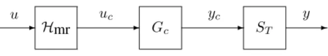
Fig. 3. Simulation result: cart position and crane angle

0 5 10 15 20 25 30

−300

−200

−100 0 100 200 300

time [sec]

input

force [N]

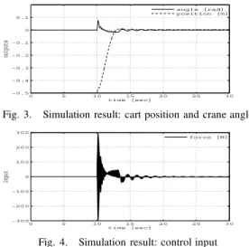
Fig. 4. Simulation result: control input

Figs. 3 and 4 show simulation results of the proposed multirate control strategy – vibration of the pendulum is effectively suppressed and the cart moves smoothly to the desired position.

V. C

ONCLUSIONS

In this paper, we proposed a robust adaptive output feedback controller design scheme for general MIMO systems using the idea of multirate sampled data control. The proposed robust adaptive control scheme negates the causality problem and can be implemented even though the controlled system has an input direct through pass.

R

EFERENCES

[1] I. Bar-Kana and H. Kaufman, “Global stability and performance of a simplified adaptive algorithm,”Int. J. Control, vol. 42, no. 6, pp. 1491–

1505, 1985.

[2] I. Bar-Kana, “Absolute stability and robust discrete adaptive control of multivariable systems,”Control and Dynamic Systems, vol. 31, pp. 157–

183, 1989.

[3] Z. Iwai and I. Mizumoto, “Realization of simple adaptive control by using parallel feedforward compensator,”Int. J. of Control, vol. 59, no. 6, pp. 1543–1565, 1994.

[4] H. Shibata and T. Kurebayashi, “New discrete-time algorithm for simple adaptive control,”Trans. of Society of Instrument and Control Engineers, vol. 31, no. 2, pp. 177–184 (in Japanese), 1995.

[5] H. Kaufman, I. Bar-Kana, and K. Sobel, “Direct adaptive control algorithms: Theory and applications (2nd ed.),” Springer-Verlag, 1998.

[6] Z. Iwai and I. Mizumoto, “Robust and simple adaptive control systems,”

Int. J. of Control, vol. 55, no. 6, pp. 1453–1470, 1992.

[7] I. Mizumoto and Z. Iwai, “Simplified adaptive model output following control for plants with unmodelled dynamics,”Int. J. of Control, vol. 64, no. 1, pp. 61–80, 1996.

[8] H. Ohtsuka, I. Mizumoto, and Z. Iwai, “A discrete sac system with parallel feedforward compensators,”Trans. of Society of Instrument and Control Engineers, vol. 34, no. 2, pp. 96–104 (in Japanese), 1998.

[9] I. Mizumoto, S. Ohdaira, T. Chen, M. Kumon, and Z. Iwai, “Adaptive output feedback control of general MIMO systems using multirate sampling,”Proc. of 44th IEEE CDC and ECC 2005, Seville, pp. 4475–

4480, 2005.

[10] G. Kranc, “Input-output analysis of multirate feedback systems,”IRE Trans. Automatic Control, vol. 3, pp. 21–28, 1957.

[11] P. Khargonekar, K. Poolla, and A. Tannenbaum, “Robust control of linear time-invariant plants using periodic compensation,”IEEE Trans.

on Automatic Control, vol. 30, pp. 1088–1096, 1985.

[12] T. Chen and L. Qiu, “H∞ design of general multirate sampled-data control systems,”Automatica, vol. 30, no. 7, pp. 1139–1152, 1994.

[13] T. Chen and B. Francis, “Optimal sampled-data control systems,” Lon- don: Springer, 1995.

[14] I. Bar-Kana, “Positive realness in multivariable stationary linear sys- tems,”J. of Franklin Institute, vol. 328, no. 4, pp. 403–417, 1991.