Japan Advanced Institute of Science and Technology Author(s) NAWAPHORN, KUHAKONGKIAT
Citation
Issue Date 2016‑09
Type Thesis or Dissertation Text version ETD
URL http://hdl.handle.net/10119/13807 Rights
Description Supervisor:山口 政之, マテリアルサイエンス研究科
, 博士
NAWAPHORN KUHAKONGKIAT
Japan Advanced Institute of Science and Technology
by
NAWAPHORN KUHAKONGKIAT
Submitted to
Japan Advanced Institute of Science and Technology in partial fulfillment of the requirements for the degree of
Doctor of Philosophy
Supervisor: Professor Dr. Masayuki Yamaguchi
School of Materials Science
Japan Advanced Institute of Science and Technology
September 2016
Referee-in-chief : Professor Dr. Masayuki Yamaguchi
Japan Advanced Institute of Science and Technology
Referees : Associate Professor Ken-ichi Shinohara
Japan Advanced Institute of Science and Technology
Associate Professor Kazuaki Matsumura
Japan Advanced Institute of Science and Technology
Associate Professor Tsutomu Hamada
Japan Advanced Institute of Science and Technology Professor Dr. Shuichi Maeda
Yamaguchi University
-i-
Preface
In multi-component system, the addition of a low-molecular-weight compound as a third component is frequently carried out to provide desirable properties of a material.
Understanding and controlling the distribution state of a third component have to be seriously considered because it decides the quality of a product. Generally, the distribution state of a third component is determined by the difference in the miscibility with each polymer, which is dependent upon the temperature. Furthermore, the distribution state may change by the interphase transfer when it is different from that in the equilibrium state.
In this thesis, the interphase transfer behavior of a low-molecular-weight compound as a third component between immiscible polymers is studied considering the effect of the ambient temperature. I hope this thesis will help to establish a new concept of the material design for multi-component polymer systems, which will lead to a novel smart material.
Nawaphorn Kuhakongkiat
-ii-
Contents
Chapter 1 General Introduction
1.1 Introduction 1
1.2 Polymer-Polymer Miscibility 4
1.2.1 Polymer blend and morphology 4
1.2.2 Thermodynamics of miscibility 5
1.2.3 Solubility parameter concept 15
1.3 Basics of Rheology 18
1.3.1 Oscillatory modulus 19
1.3.1 Rheological four regions 20
1.4 Elastomer Blend 22
1.4.1 Distribution of third component in immiscible elastomer blend 23
1.4.2 Transfer of curatives 23
1.4.2.1 Blooming 24
1.4.2.2 Diffusion 24
1.5 Characterization of Transfer Process 27
1.4.1 Diffusion theory 27
1.6 Objective of This Research 31
References 34
-iii-
Chapter 2 Interphase Transfer of Plasticizer between Immiscible Rubbers
2.1 Introduction 41
2.2 Experimental 42
2.2.1 Materials 42
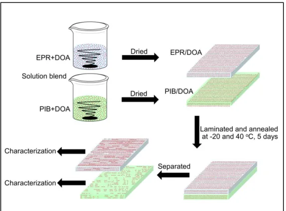
2.2.2 Sample preparation 43
2.2.3 Measurements 44
2.3 Results and Discussion 45
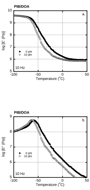
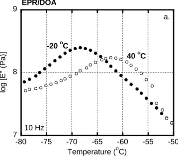
2.3.1 Role of plasticizer on the rubbers 45
2.3.2 Interphase transfer of the plasticizer 49
2.3.3 The determination of the Flory-Huggins interaction parameter 54
2.4 Conclusion 61
References 62
Chapter 3 Interphase Transfer of Tackifier between Immiscible Rubbers
3.1 Introduction 653.2 Experimental 66
3.2.1 Materials 66
3.2.2 Sample preparation 67
3.2.3 Measurements 68
3.3 Results and Discussion 68
3.3.1 Characteristics of rubbers containing tackifie 68
-iv-
3.3.2 Interphase transfer of the plasticizer 74
3.4 Conclusion 79
References 80
Chapter 4 Thermochromic Immiscible Polymer Blend by Interphase Transfer of Plasticizer
4.1 Introduction 834.2 Experimental 84
4.2.1 Materials 84
4.2.2 Sample preparation 85
4.2.3 Measurements 86
4.3 Results and Discussion 87
4.3.1 Effect of the plasticizer addition 87
4.3.2 Interphase transfer of DOA 92
4.3.3 Structure and properties of blends 95
4.4 Conclusion 99
References 100
Chapter 5 General Conclusion 101
Achievements 105
Minor Research Theme 109
Acknowledgements 139
- 1 -
Chapter 1
General Introduction
1.1 Introduction
The science and technology of polymeric materials have been significantly developed due to their unique properties and light weight, and further development is expected to meet a demand of various applications [1-4]. Research activities in the past have been concentrated mainly on the chemical approach such as catalyst and polymerization techniques. Since these routes have become increasingly complex and lead to poor cost performance, blending, as an alternative technique, has been focused these days.
Some of polymer blends have been successfully commercialized with the combination of excellent properties, which cannot be attained from one polymer species.
This strategy is known as one of the powerful approaches with the advantages of good cost performance and easy processing. Additionally, polymer blends can cover a wide range of material properties by changing the blend composition.
Polymer blends are of great importance also in the rubber industry, especially for automotive and transportation applications [5-8]. It is an effective and economic approach to satisfy the divergent requirements of properties compared to synthesizing new elastomers.
Prospestive commitments of rubber blends are (1) product uniformity, (2) good processability, (3) efficient productivity, and (4) rapid formulation changes and manufacture flexibility. Moreover, the addition of a low-molecular-weight additive has been often carried
- 2 -
out to satisfy properties for a final product. For example, the addition of curatives such as sulfur to create a three-dimensional network vulcanization [9] and a processing oil to provide flexibility and processability [10].
Because commercial rubbers have generally high molecular weight, their blends are typically not miscible due to the lack of the contribution of mixing entropy as explained later. In the case of an immiscible polymer blend containing a low-molecular-weight compound as a third component, the overall phase-separated morphology is governed by not only the properties of individual components, but also the interaction among them. In particular, the distribution state of a low-molecular-weight compound is determined by the difference in the miscibility with each rubber component, which is expressed by the Flory- Huggins interaction parameter [11, 12]. In general, a third component prefers to reside in a polymer component with the low interaction parameter. In addition, the interaction parameter is dependent upon the ambient temperature, pressure and flow field. In other words, the distribution state of a low-molecular-weight additive in a blend changes with these conditions.
Moreover, the distribution state may change during storage. In fact, some researchers have reported that the distribution state of a compound in an immiscible rubber blend changes by the interphase transfer phenomenon. Since the factors controlling the distribution, e.g., the interaction parameter, is a function of the temperature, the preferable distribution state of a third component can be controlled by the ambient temperature when the diffusion is allowed for a third component. In this case, the amount of a third component in each phase changes with the ambient temperature. This will lead to a novel material
- 3 -
design. In this thesis, the effect of the temperature on the distribution will be focused, which has not been carried out before to the best of my knowledge.
This chapter covers the background information prior to the discussion on the transfer phenomenon. The fundamental of miscibility of a polymer blend, the rubber technology, and the distribution of a low-molecular-weight compound in a rubber blend are explained in the combination with literature reviews. Finally, the objective of the thesis is mentioned.
- 4 - 1.2 Polymer-Polymer Miscibility
1.2.1 Polymer blend and morphology
Processability and mechanical properties of a polymer blend are strongly dependent on morphology [3, 13]. Therefore, the control of morphology is the key factor in the field of polymer blends. Most polymer blend systems are immiscible and exhibit phase-separated morphology. Two notable morphologies for immiscible blends are co-continuous morphology and sea-island morphology, which can be characterized by various methods [14-17]. The morphology of an immiscible polymer blend depends on (1) mixing procedure, (2) rheological properties of the components, and (3) interfacial tension.
The mixing process is the first step to control the morphology. The model mechanism was initially proposed by Scott and Macosko [18, 19], in which the shape of the dispersed amorphous polyamide is deformed from spheres to platelets under the shear field in the polystyrene matrix as shown in Figure 1.1. Their experimental results demonstrated the morphology development at the processing. Jordhamo et al. [20] noted the essential condition to create co-continuous morphology as follows;
1
1 2
2
1
(1.1)
where η1, η2 and θ1, θ2 are the viscosity and weight fraction of each component in the blend.
- 5 -
Figure 1.1 Morphology development of a polymer blend at mixing process. [18]
1.2.2 Thermodynamics of miscibility
The structure of a polymer blend is primarily determined by the miscibility of the components. In the equilibrium state, the miscibility is governed by the Gibbs free energy of mixing ΔGm [21];
m m
m H T S
G
(1.2)
whereHmis the enthalpy of mixing (heat of mixing), and Smis the entropy of mixing determined by the Boltzmann relationship. Since the entropy term is negligible for polymer blends, Hmis the key factor to decide the miscibility.
- 6 -
Assuming that ΔSm is zero, the miscibility is determined by ΔHm, as follows.
1. Miscible blend: ΔHm is negative due to the specific interaction between components, e.g., ion-dipole interaction, hydrogen bond, etc. Both components are dissolved together in a molecular scale.
2. Immiscible blend: ΔHm is positive. The phase separated morphology is observed.
The miscibility is, of course, affected by the mixing entropy. This becomes very important when components have low molecular weight. For a polymer-polymer blend, Sm is small because of the high molecular weights. The assumption in the Flory-Huggins theory based on the lattice model [11, 12, 22, 23] is applied to determine the entropy of mixing for the mixture as illustrated in Figure 1.2.
Figure 1.2 Lattice model for (a) solvent-solvent blend, (b) solvent-polymer blend, and (c) polymer-polymer blend.
- 7 -
From the figure, the lattice is comprised of N cells with a volume of v. Each cell is occupied by one segment of any molecule. The entropy change of mixing can be derived through the number of cites of a lattice as follows;
) ln ln
(N1 1 N2 2 k
Sm B
(1.3)
) ln ln
( 2
2 2 1 1
1
r V r
k
Sm B
(molecular basis) (1.4)
) ln ln
( 2
2 2 1 1
1
r RV r
Sm
(molar basis) (1.5)
where kB is the Boltzmann constant, V is the total volume, R is the gas constant, and ϕi and ri are the volume fraction and the number of polymer segment i.
As mentioned that most polymer pairs have a small value of ΔSm. Therefore, the miscibility is usually determined by the contribution of ΔHm. The term of enthalpy change has relation with the Flory-Huggins interaction parameter χ12 by the following equation.
r
m RTV v
H 12 12
(1.6)
wherevr is the reference volume.
Consequently, the following two expressions are obtained to express the Gibbs free energy of mixing.
r B B
m k TV v
r TV r
k
G ln ln 2 1 2 12 /
2 2 1 1
1
(molecular basis) (1.7)
r
m RTV v
r RTV r
G ln ln 2 1 2 12 /
2 2 1 1
1
(molar basis) (1.8)
- 8 -
The general style of the Flory-Huggins equation is given;
r V RTV r
Gm 2 12 1 2
2 2 2 1 1
1
1 ln ln
(1.9)
where ρi is the density of the component i.
Finally, the following equation is obtained, assuming ρ1 = ρ2 = 1.
2 12 1 2
2 2 1 1
1 ln ln
r RT r
V Gm
(1.10)
It has been reported that most polymer pairs have positive ΔHm. Consequently, there are a lot of immiscible systems. In other words, two polymers can be miscible only when they have specific interactions between the components (ΔHm < 0), e.g., hydrogen bonding and ion-dipole interaction.
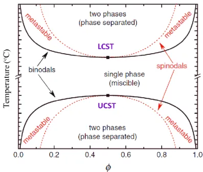
There are two famous critical temperatures to illustrate a phase diagram of a polymer blend, i.e., upper critical solution temperature (UCST) and lower critical solution temperature (LCST). The phase diagram including the critical temperature is illustrated in Figure 1.3, in which the blend ratio and the temperature are the variables.
- 9 -
Figure 1.3 Phase diagram showing LCST and UCST behavior for blend systems.
In the classical lattice theory, polymer blends can show only UCST but not LCST, because χ12 is given as follows;
k T
z
B
12 (molecular basis) or (1.11)
RT z
12 (molar basis) (1.12)
where z is the coordinate number of the lattice model.
The term of ∆ε is the difference in the interaction energies between chain segments of components, which is derived from the relationship;
11 22
122
1
(1.13)
where εij is the constant energy of contacts between components i and j.
- 10 -
Then, the Flory-Huggins interaction parameter can be written as follows;
)
( 112 12 12
12
T k
z
B
(molecular basis) or (1.14)
2 )
( 11 12 12
12
RT
z (molar basis) (1.15)
In 1960, Freeman and Rowlinson found that several hydrocarbon polymers can be dissolved in hydrocarbon solvents [24]. These nonpolar polymer solutions exhibited the phase separation at high temperature, known as LCST behavior. This seldom happens in a mixture of low-molecular-weight compounds. Of course, the original Flory-Huggins theory assuming eq. (1.11) and (1.12) cannot describe the phenomenon. Flory and co-workers [25- 31] then developed the new theory for the solutions, which can predict the LCST behavior.
Furthermore, various models have been proposed such as the Prigogine-Flory-Patterson theory [27, 32-34], the lattice-with-holes theory [35, 36], and Sanchez-Lacombe lattice fluid model [37, 38]. They are called “equations of state theories”.
The equation of state is basically a mathematical relationship between volume, temperature, and pressure, which can be written by three parameters: v* (characteristic reduced volume), T* (characteristic reduced temperature), and P* (characteristic reduced pressure). The reduced variables are defined as
/ *
~ T T
T (1.16)
/ *
~ P P
P (1.17)
/ *
~ v v
v (1.18)
- 11 -
The volume v* is that of a polymer segment and v is the actual volume of a segment.
Thus ṽ is the reduced value per segment. The values of ṽ and P͂ were estimated by thermal expansion coefficient. The Flory-Huggins interaction parameter χ12 can be expressed using the reduced variables as follows;
2
* 2
* 1 3
/ 1 1 3 / 1 1
* 1 3 / 1 1
12 3 / 1 1
* 1
* 1 ,
1 1
12 1
~ 3 2 4
~
~ 1
~
~ T
T v
v P
v X v RT
P v
M sp
(1.19)
where M1 is the molecular weight of a polymer and X12 is an exchange interaction parameter between polymer and solvent.
The interaction term X12 is similar to χ12 in the Flory lattice theory, but has the dimensions of energy density as given by;
12 2 1
* 2 2
* 1 1
* P P X
P (1.20)
where ϕi is the volume fraction of component i and θ2 is the segment surface fraction.
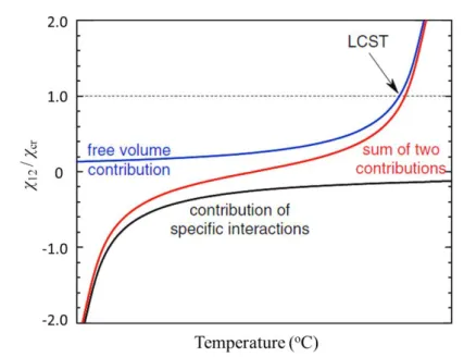
In the modified theory, the following three principle contributions are important for the interaction parameter, i.e, dispersion force contribution, free volume contribution, and the contribution of specific interaction. In general, the dispersive force and specific interaction are inversely proportional to temperature as shown in eqs. (1.14) and (1.15), whereas the contribution of free volume is always increasing with temperature as a positive value. These two opposite contributions are responsible for the LCST behavior as shown in Figure 1.4.
- 12 -
Figure 1.4 Schematic diagram of the UCST and LCST phase diagrams for liquid mixtures relating to the free energy of mixing contributions
The miscibility can only be achieved when χ12 is lower than χcr, where χcr is the maximum value (> 0) to show the miscibility. The dotted line (χ12/ χcr = 1) is the temperature at which the miscibility changes. Furthermore, χcr can be obtained as follows;
2
2 / 1 2 2 / 1 1
1 1 2
1
r r
cr
(1.21)
where ρ is the average density.
- 13 -
When the specific interactions such as hydrogen bonding and electrostatic interactions governs the miscibility, the phase diagram is written in Figure 1.5.
Figure 1.5 LCST phase behavior of polymer blend controlling the interaction parameter by the contribution of the specific interactions
The free volume contribution was explained by using other characteristics of polymer chains. Lohse et al. studied the miscibility of saturated hydrocarbon elastomer blends using small-angle neutron scattering and PVT measurements [39, 40]. The PVT data provide the cohesive energy density CED = U/V , which has a close relation with the internal pressure ΠIP = ∂U/∂V. This parameter depends on not only the chemical composition, but also their chain packing density.
The packing length is defined as the ratio of the occupied volume Vocc of the chain, defined by eq. (1.22), to the radius of gyration rg. Vocc is the occupied volume of a unit polymer, which is directly defined by the polymer density.
- 14 -
A
OCC N
V M
(1.22)
where NA and M are the Avogadro’s number and molecular weight of a component, respectively.
Since the average of rg2 in the melt is proportional to M, Vocc/rg2 is independent of the molecular weight, the packing length lp is defined as follows;
A g g OCC
p r N
M r
l V
2
2
(1.23)
It has been reported that the packing length is correlated with the solubility parameter by the following expression;
2 / 1
3
0
1 2 2
a l a m
N
p A
(1.24)
where m0 is the molecular weight of a repeating unit. The parameters a and ε represent the length and energy scales of the component associated with the entanglement spacing.
The solubility parameter is inversely proportional to the packing length as long as both a and ε are constant. In other words, a smaller packing length provides a large solubility parameter. This is reasonable because small packing length leads to large radius of gyration, which can overlap the neighboring polymer chains with a strong interaction. The difference in the packing length is, therefore, used to predict the miscibility of non-polar systems [41- 44].
- 15 - 1.2.3 Solubility parameter concept
The solubility parameter is known as a conventional parameter to predict the miscibility. When two materials have similar solubility parameters, then they may be miscible. This concept was firstly introduced by Scatchard [45], who defined the cohesive energy density as the energy of evaporation Ev per unit volume. Then Hildebrand and Scott [46] further developed to obtain the following equation;
1/2 1/2
V
CED Ev
(1.25)
The value is noted to be influenced by the specific solvent internal pressure [47]. For most of low-molecular-weight materials, e.g., organic liquids, the value can be estimated by several sources such as the heat of evaporization. In the case of high-molecular-weight polymers, the heat of evaporation cannot be measured directly. Therefore, the solubility parameter is typically estimated by viscosity or swelling of a crosslinked sample in a series of solvents.
Hansen [48] further considered the solubility parameter using three components, i.e., dispersion interaction δd, polarity δp, and hydrogen bonding δh. The total solubility parameter δt is given by the root mean square of these components.
2 2 2 2
h p d
t
(1.26)
Another approach has been used to predict the solubility parameter without physical experiments, which is known as the group contribution method, firstly developed by Small [49]. This method was further developed by van Krevelan [50], Hoy [51], and Coleman [52].
- 16 -
For this method, values of molar attraction constants are required as illustrated in Figure 1.6. The Small’s formula is given by;
M GMi
t
(1.27)
where ρ is the density,
Σ
GMi is the summation of the molar attraction constants of i-group, and M is the molar mass of a repeating unit.Figure 1.6 Group molar attraction constants [49]
- 17 -
The Flory-Huggins interaction parameter χ12 is an important tool for quantifying the degree of miscibility for polymers. It can be presented with the correlation with the solubility parameters by combining Hidebrand-Scatchard solution theory as follows;
1 2
212
RT
V (1.28)
Based on this equation, however, the interaction parameter never become a negative value. Although this situation is not correct, the calculated value can be used to predict the miscibility roughly.
As seen in eq. (1.25), the solubility parameter is the square root of the cohesive energy density of the pure liquid. In the case of nonpolar liquid, i.e., saturated hydrocarbon, the cohesive energy is related approximately to its internal pressure. It can be determined by PVT measurements, which leads to;
2 / 1
) (
) (
T T T
PVT
(1.29)
where α is the thermal expansion coefficient of a liquid and β is the isothermal compressability.
As mentioned, a solubility parameter is dependent upon the temperature. Table 1.1 shows the PVT results of several polyolefin materials at various temperatures.
- 18 -
Table 1.1 Characteristic components on PVT data for several polyolefin materials [53]
Species T
(oC)
α (T) x 104 (K-1)
β (T) x 104 (MPa-1)
δPVT (T) (MPa 1/2)
PP
atactic polypropylene
27 51 83 121 167
7.28 7.55 7.31 7.30 7.52
6.47 7.54 8.73 10.44 13.14
18.37 18.02 17.25 16.60 15.87 EP57
copolymer of ethylene and propylene (23 wt.% propylene)
27 51 83 121 167
6.77 7.06 7.12 7.41 8.10
5.89 6.88 7.87 9.28 11.49
18.57 18.24 17.94 17.73 17.61 PEP
alternating copolymer of ethylene ad
propylene
27 51 83 121 167
6.60 6.78 6.69 6.88 7.33
5.82 6.74 7.87 9.30 11.50
18.45 18.06 17.39 17.07 16.74 PIB
polyisobutylene
27 51 83 121 167
5.52 5.72 5.53 5.68 6.08
4.80 5.52 6.29 7.41 8.85
18.58 18.33 17.68 17.38 17.38
1.3 Basics of Rheology
Rheology is a science of the deformation and flow. Therefore, elastic and viscous properties are frequently dealt in this field. In general, most polymer melts exhibit both elastic and viscous responses, i.e., viscoelasticity. The elastic response of a polymer liquid is attributed to the entanglement couplings of long molecules.
Hooke’s law is applicable to a perfect elastic body by the following equation.
E (1.30)
where σ and ε are the stress and strain, respectively and E is the modulus.
- 19 -
Viscosity expresses the resistance to flow. Following the Newton’s law, viscosity η is defined as the ratio of the stress (σ = F/A) and strain rate ε̇ as follows;
(1.31)
1.3.1 Oscillatory modulus
The response of dynamic oscillatory stress and strain is expressed in Figure 1.7.
Figure 1.7 Sinusoidal oscillating stress and strain with a phase angle δ
The sinusoidal response with strain as a function of angular frequency ω, given by the following expressions;
) sin(
)
( 0
t t (1.32)
) sin(
)
(t 0 t
(1.33)
where δ (0 ≤ δ ≤ π/2) is a phase lag of the response.
- 20 -
When an oscillatory deformation ( 0eit) is applied to a viscoelastic body, the stress is generated as follows;
E*( ) (1.34)
E( )iE( ) (1.35)
where E*(ω) is complex modulus, E' is elastic storage modulus, and E'' is viscous loss modulus.
The complex modulus is given by;
z E i z
z E
E z2 2 2 2
2 2
*
1
1
(1.36)
where z is the relaxation time.
E i E
E* (1.37)
E E
tan (1.38)
1.3.2 Rheological four regions
Temperature dependence of viscoelastic behaviors is shown in Figure 1.8. In general, a polymer has four regions such as glassy region, transition region, rubbery region, and flow region from the low temperature.
- 21 -
Figure 1.8 Four regions of an amorphous polymer
In the glassy region, Brownian motion is prohibited and only vibrations and short- range rotational motions are allowed. This region is observed in the low temperature range or high frequencies. Young’s modulus is around 109-1010 Pa.
In the glass-to-rubber transition region, the Brownian motion starts to occur. The modulus is 106-1010 Pa and drops off greatly in a narrow temperature range. In this region, the glass transition temperature Tg is the important physical property, which can be defined as the peak temperature of loss modulus E''.
Beyond Tg, the modulus becomes almost a constant (105-106 Pa as a tensile modulus), known as the rubbery plateau modulus. In this region, Brownian motion is allowed between entanglement couplings. In other words, entanglement couplings act as crosslink points. The length of the plateau is dependent on the molecular weight. The molecular weight between entanglements Me can be evaluated from the modulus at the rubbery plateau GN0 by the following equation using the classical rubber theory.
- 22 -
0 N
e G
M RT
(1.39)
In the flow region, the relaxation time associated with entanglement couplings is shorter than the observation time. Consequently, a material shows viscous flow. Although elastic properties are still detected, viscosity is a dominant characteristic for mechanical behaviors of a polymer.
1.4 Elastomer Blend
Conventional unsaturated elastomers, e.g., natural rubber (NR), synthetic polybutadiene (BR), and poly(styrene-co-butadiene) rubber (SBR), are commercially important in the automotive tire manufactures. However, they are usually used in blends to satisfy the properties, e.g., chemical, physical, and processing benefits for each application [54-57].
Table 1.2 lists the important components of tire and the typical blends used for them.
It is known that most rubber blends show phase-separated morphology because of their high molecular weight.
- 23 -
Table 1.2 Elastomer blends for automotive tires [58, 59]
Passenger tires Truck tires
Tread SBR-BR NR-BR or
SBR-BR
Belt NR NR
Carcass NR-SBR-BR NR-BR
Sidewall NR-BR or
NR-SBR NR-BR
Liner NR-SBR-IIR NR-IIR
IIR = isobutylene-isoprene rubber or butyl rubber
1.4.1 Distribution of third component in immiscible elastomer blend
Various compounds are added in rubber blends as a third component, including plasticizers, processing oil, antioxidants, and vulcanizing agents. Their distribution state dramatically influences properties of a final product as well as the processability.
Rubber compounds are mixed in the highly viscous state above their glass transition temperatures, in which additives may be distributed in one component or at the interface.
Besides, the transfer phenomenon from one phase to another may occur during mixing and/or post-processing annealing. Therefore, it is significantly important for the material design to select an appropriate third component in each rubber blend.
1.4.2 Transfer of curatives
Sulfur is often used as a crosskinking agent especially for unsaturated rubbers, while peroxide system is used for saturated rubbers. Activators and accelerators are other kinds of ingredients to promote crosslinking without side reactions. The distribution of these
- 24 -
curatives is significantly important for rubber blends to control the mechanical properties.
Curatives are initially located within a continuous phase at mixing. However, the difference in the miscility leads to the uneven distribution. Because most curatives are composed of polar molecules, they preferably reside in a polar rubber. When the distribution state after mixing is far from that in the equilibrium, the transfer through the interface may take place as demonstrated by a number of researchers [60-63].
1.4.2.1 Blooming
This is not a transfer from one rubber to another, but the diffusion from a rubber to outside. It occurs when the amount is beyond the critical volume at a given temperature. One example is the migration of sulfur to the surface, which is eventually crystallized [64].
Therefore, a patent to use specific sulfur in a particular compound was filed to eliminate blooming [65]. Mastromatteo et al. [66] reported that the use of accelerators with longer alkyl chains can provide non-blooming cure system for ethylene-propylene diene momomer (EPDM) and results in good physical properties of acrylonitrile-butadiene rubber (NBR) blend with EPDM.
1.4.2.2 Diffusion
When the solubility of curatives is limited, the diffusion occurs to be in the equilibrium condition. Gardiner [61, 62] showed that conventional curatives usually diffuse from less polar rubber to more polar one across the boundary of phases, which occurs very
- 25 -
quickly during both mixing and vulcanization procedures. He estimated the diffusion coefficient from the concentration changes as a function of distance and time. The diffusion coefficients of sulfur and accelerators from isobutylene-isoprene rubber or butyl rubber (IIR) to other rubbers are listed in Table 1.3.
Table 1.3 Interphase transfer of curatives in elastomer blends
Curatives From To Diffusion coefficient,
D x 107 (cm2/s)
Accelerator (TDDC) IIR BR 12.66
EPDM 1.09
CR 1.08
SBR 0.58
NR 0.70
Sulfur IIR SBR 4.73
SBR & 50PHR
N700 CB 17.2
NR 2.82
TDDC = Tellurium diehyldithiocarbamate CR = Polychloroprene or chloroprene rubber N700 CB = reinforcing type carbon black
In many cases in industry, co-vulcanization is required, e.g., a blend of EPDM and unsaturated rubbers, at which the curative distribution is a key technology to provide more uniform crosslinking. Grafting of accelerators onto EPDM prior to blending or addition of a long-chain dithiocarbamate are alternative ways to improve both co-crosslinking and compatibility [67].
The large difference in the solubility parameter leads to the rapid transfer of curatives at the vulcanization temperature. In order to prevent the lack of co-vulcanization in the
- 26 -
blends, the accelerators with the same difference in the solubility parameter with each rubber component should be added [68]. Attempts to determine the solubility parameters of sulfur and accelerators have been carried out for a long time [64, 68-71]. The solubilities of several curatives and rubbers are given in Figure 1.9.
CBS = N-cyclohexylbenzothiazole-2-sulphenamide DCBS = N-dicyclohexylbenzothiazole-2-sulphenamide IS = insoluble sulfur
MBT = 2-mercaptobenzothiazole
S8 = eight-membered ring sulfur or octasulfur
Figure 1.9 Solubility parameter [(MPa)1/2] of various rubbers and some curatives. [71]
Besides fillers and curatives, the transfer of other additives such as wax, antioxidant, antiozonant, processing oil, and plasticizer, also play an important role in the properties of a blend [10, 72-75]. In the rubber formulation, petroleum wax can cause the transfer and/or blooming, as similar to sulfur. The wax blooming is, however, used to protect a vulcanized rubber surface against ozone attack due to the carbon-carbon double bond (C=C) of elastomer chains. Lewis et al. [63] showed that antiozonants prefers to migrate from EPDM to SBR during curing. It has been reported that the extent of migration depends on not only solubility, but also mobility of wax. The latter is affected by rubber composition and the ozone exposure conditions, such as time and temperature [76, 77].
- 27 -
The primary role of oil and plasticizer is to increase flexibility of polymeric chains and to improve the rheological properties suitable for processing operations by lowering the glass transition temperature Tg and viscosity. Oil and plasticizer are dissolved into rubber with no chemically bonding and act as an internal lubricant. However, bleeding out may occur for these additives with poor miscibility.
In addition, the tackifier is another type of low-molecular-weight compounds with high softening point, which commonly enhances the adhesion of vulcanized rubbers.
According to Basak et al. [78], good adhesion between the vulcanized and unvulcanized EPDM is improved by the addition of a tackifier, which can be explained by the “single side interdiffuion” concept. Doan et al. [79] found that the tackifier transfer occurs from BR to SBR due to the miscibility difference.
1.5 Characterization of Transfer Process 1.5.1 Diffusion theory
As well known, Einstein developed and established the theory of Brownian motion in 1905 [80, 81]. Diffusion of spherical particles is expressed by the following relation;
D t
r( )2 6
(1.40)
Tb k
D B (1.41)
- 28 -
where r(t)2 is the mean-square displacement, D is the diffusion coefficient, kB is the Boltzmann constant, b is the mobility constant of a particle or segment, and T is the absolute temperature.
Einstein also showed that the diffusion coefficient is inversely proportional to the friction coefficient ξ, known as the Nernst-Einstein relation.
T
Dr kB (1.42)
In the case of large particles, there is no tendency for the solution to slip at the surface of the spherical particle. The value of ξ can be obtained by the Stokes law as follows;
R
6 (1.43)
where R is the radius of particles and η is the viscosity of a medium.
By combining the Nernst-Einstein relation and the Stokes law, the following equation is given [82];
R T Dr kB
6 (1.44)
This equation is widely used to explain the diffusion of a spherical nanoparticles, whose radius is larger than the radius of gyration of a polymer chains [83-85].
The presence of a liquid fraction is significant importance for rheological and physical properties. During compounding, liquids may penetrate from one rubber to another acrossing the boundary of interphase, which is described by the Fick’s law of diffusion. The diffusion process is characterized by a dimensionless parameter called the Deborah number
- 29 -
for diffusion Db. This number is defined as a ratio of the characteristic time of a fluid λf to the characteristic time for the diffusion process θD [86].
D f
Db
(1.45)
The diffusion of small molecules in a polymer or in a network of highly entangled chains is often observed at a temperature well above Tg, leading to the small value of Deborah number of diffusion. At this state, the diffusion process is classified into Fickian type based on the rate of diffusion. The Fick’s first law says that the flow of molecules or mass flux J is proportional to the concentration gradient [87];
x D c
J
(1.46)
where D is the mass diffusion coefficient [m2 s-1] and x c
is the concentration gradient.
The Fick’s second law expresses the time evolution of the concentration profile, which is obtained from the mass balance of a diffusing molecule in a unit volume [88];
2 2
x D c t c
(1.47)
x D c c t
c (1.48)
When the diffusion process occurs through a flat sheet of thickness l, whose surfaces are maintained at constant concentrations c1 and c2, the steady state is reached when the concentration in the sheet is constant;
2 0
2
x
c (1.49)
- 30 -
x
c constant (1.50)
By further integration at the conditions of x=0 and x=l, it can be written by;
1 1
2 x c
l c
c c
(1.51)
leading to
l c Dc x D c
J 1 2
(1.52)
The diffusion coefficient in a polymer matrix with molecular weight of M is described by a power law [89].
KM
D (1.53)
where K and α are constants.
The value of the exponent α was reported to be 2 [90, 91]. Moreover, the diffusion coefficient is a function of temperature, which is expressed by the Arrhenius equation.
RT
D E
D 0exp D (1.54)
where D0 is the pre-exponential factor and ED is the activation energy of the diffusion. The experimental results revealed that ED is given by the following equation;
v
D d E
E 2 (1.55)
where d is the diameter of a molecule and ΔEv is the cohesive energy [92, 93];
The diffusion in a polymer is accelerated by sufficient free volume in the molten state [94, 95], because penetrant molecules can migrate only in a free space. Therefore, the diffusion is accelerated in a polymer with a number of chain ends, i.e., low molecular
- 31 -
weight. Moreover, the crystallinity and temperature are the factors influencing the diffusivity.
The diffusion occurs significantly slow below the glass transition temperature Tg [96, 97]. At this temperature, the free volume fraction, i.e., Vf /(Vf +Vo), is believed to be 2.5%.
Beyond Tg, the free volume fraction increases rapidly with temperature as illustrated in Figure 1.10.
Figure 1.10 Temperature dependence of occupied volume (Vo) and free volume (Vf)
1.6 Objective of This Research
For a multi-component system, especially for an immiscible polymer blend, the addition of a low-molecular-weight compound as a third component is a significant importance to provide required properties of a final product. The distribution state of a third
- 32 -
component is generally determined by the miscibility between a third component and each polymer, which can be changed by ambient temperature.
The transfer phenomenon of a third component between dissimilar polymers can occur from one phase to another through the boundary of the phases. This will lead to the uneven distribution of this component in the blend, which depends upon the temperature.
Previous researches on the transfer phenomenon were carried out at a fixed temperature, which is significantly different from my research.
The main objective of this research is to study “the temperature dependence of the distribution state of various types of liquid compounds in an immiscible polymer blend”, as well as the interphase transfer phenomenon between immiscible polymers. The difference in the miscibility as a function of temperature will be discussed using solubility parameter and Flory-Huggins interaction parameter. It should be underlined that Tg is determined by a liquid concentration. Therefore, it is expected to control Tg of each phase when the amount of a liquid can change with ambient temperature.
At first, in the following Chapter 2, a plasticizer was introduced in a binary polyolefin elastomer blend, which is composed of ethylene-propylene copolymer and poly(isobutylene). The interphase transfer due to the difference in the temperature dependence of the Flory-Huggins interaction parameter is discussed. Then the transfer of a coumarone-indene tackifier between immiscible conventional rubbers, such as natural rubber and poly(isobutylene), was investigated in Chapter 3. In this chapter, the crystallization of NR is found to accelerate the tackifier transfer at low temperature. Furthermore, controlling transparency driven by the interphase transfer of a low-molecular-weight compound with
- 33 -
low refractive index between ethylene-vinyl acetate copolymer and poly(vinyl butyral) is discussed in Chapter 4. Finally, the details of this research are summarized in Chapter 5.
Through this research, a better understanding of the interphase transfer of a third component is expected. Furthermore, the uneven distribution of a third component in an immiscible blend can be precisely controlled by the ambient temperature. This would be applicable to the development of a high-performance immiscible polymeric materials.
- 34 - References
1. Paul, D. R.; Newman, S., Polymer Blends. Academic Press: New York, 1978.
2. Robeson, L. M., Polymer Engineering & Science 1984, 24 (8), 587-597.
3. Utracki, L. A., Polymer Blends Handbook. Springer Netherlands: Dordrecht, 2003.
4. Vaia, R. A.; Giannelis, E. P., MRS Bulletin 2001, 26 (05), 394-401.
5. Cheremisinoff, N. P.; Cheremisinoff, P. N., Elastomer Technology Handbook. CRC Press: Florida, 1993.
6. De, S. K.; White, J. R., Rubber Technologist's Handbook. Rapra Technology Limited: 2001.
7. Findik, F.; Yilmaz, R.; Köksal, T., Materials & Design 2004, 25 (4), 269-276.
8. Feng, W. I., A. I., Journal of Materials Science 2005, 40 (11), 2883-2889.
9. Noriman, N. Z.; Ismail, H.; Rashid, A., Polymer-Plastics Technology and Engineering 2008, 47 (10), 1016-1023.
10. Nakason, C.; Kaewsakul, W., Journal of Applied Polymer Science 2010, 115 (1), 540-548.
11. Flory, P. J., The Journal of Chemical Physics 1942, 10 (1), 51-61.
12. Huggins, M. L., The Journal of Physical Chemistry 1942, 46 (1), 151-158.
13. Alfrey, T. S., W. J., Science 1980, 208 (23), 813-818.
14. Kumar, C. R.; George, K. E.; Thomas, S., Journal of Applied Polymer Science 1996, 61 (13), 2383-2396.
15. Schuster, R. H., Macromolecular Symposia 2002, 189 (1), 59-81.
16. Tsou, A.; Waddell, W., Kautschuk und Gummi Kunstoffe 2002, 55 (7/8), 382-387.
- 35 -
17. Rocha, T.; Rosca, C.; Ziegler, J.; Schuster, R., Kautschuk Gummi Kunststoffe 2005, 58 (1-2), 22-22.
18. Scott, C. E.; Macosko, C. W., Polymer 1994, 35 (25), 5422-5433.
19. Scott, C. E.; Macosko, C. W., Polymer 1995, 36 (3), 461-470.
20. Jordhamo, G. M.; Manson, J. A.; Sperling, L. H., Polymer Engineering & Science 1986, 26 (8), 517-524.
21. Gibbs, J. W., Transactions of the Connecticut Academy of Arts and Sciences 1873, 2, 382-404.
22. Flory, P. J., The Journal of Chemical Physics 1941, 9 (8), 660-660.
23. Huggins, M. L., Journal of the American Chemical Society 1942, 64 (7), 1712-1719.
24. Freeman, P. I.; Rowlinson, J. S., Polymer 1960, 1, 20-26.
25. Flory, P. J.; Orwoll, R. A.; Vrij, A., Journal of the American Chemical Society 1964, 86 (17), 3507-3514.
26. Flory, P. J.; Orwoll, R. A.; Vrij, A., Journal of the American Chemical Society 1964, 86 (17), 3515-3520.
27. Flory, P. J., Journal of the American Chemical Society 1965, 87 (9), 1833-1838.
28. Eichinger, B. E.; Flory, P. J., Transactions of the Faraday Society 1968, 64 (0), 2035-2052.
29. Eichinger, B. E.; Flory, P. J., Transactions of the Faraday Society 1968, 64 (0), 2053-2060.
30. Eichinger, B. E.; Flory, P. J., Transactions of the Faraday Society 1968, 64 (0), 2061-2065.
- 36 -
31. Eichinger, B. E.; Flory, P. J., Transactions of the Faraday Society 1968, 64 (0), 2066-2072.
32. Prigogine, I.; Trappeniers, N.; Mathot, V., Discussions of the Faraday Society 1953, 15 (0), 93-107.
33. Prigogine, I., The Molecular Theory of Solutions. North-Holland Publishing Company: New York, 1957.
34. Patterson, D., Macromolecules 1969, 2 (6), 672-677.
35. Simha, R.; Havlik, A. J., Journal of the American Chemical Society 1964, 86 (2), 197-204.
36. Bonner, D. C.; Bellemans, A.; Prausnitz, J. M., Journal of Polymer Science Part C:
Polymer Symposia 1972, 39 (1), 1-9.
37. Sanchez, I. C.; Lacombe, R. H., The Journal of Physical Chemistry 1976, 80 (21), 2352-2362.
38. Panayiotou, C.; Sanchez, I. C., Macromolecules 1991, 24 (23), 6231-6237.
39. L. J. Fetters; D . J. Lohse; D. Richter; T . A. Witten; Zirkelt, A., Macromolecules 1994, 27 (17), 4639-3647.
40. Lohse, D. J.; Garner, R. T.; Graessley, W. W.; Krishnamoorti, R., Rubber Chemistry and Technology 1999, 72 (4), 569-579.
41. Lewis J. Fetters; David J. Lohse; Scott T. Milner; Graessley, W. W., Macromolecules 1999, 32 (20), 6847-6851.
42. Lohse, D. J., Journal of Macromolecular Science, Part C: Polymer Reviews 2005, 45 (4), 289-308.
- 37 -
43. White, R. P.; Lipson, J. E. G.; Higgins, J. S., Macromolecules 2012, 45 (2), 1076- 1084.
44. White, R. P.; Lipson, J. E. G., Macromolecules 2014, 47 (12), 3959-3968.
45. Scatchard, G., Chemical Reviews 1931, 8 (2), 321-333.
46. Hildebrand, J. H.; Scott, R. L., The Solubility of Nonelectrolytes. Reinhold: New York, 1950.
47. Hildebrand, J. H., Journal of the American Chemical Society 1916, 38 (8), 1452- 1473.
48. Hansen, C. M., Journal Paint Technology 1967, 39 (505), 104-117.
49. Small, P. A., Journal of Applied Chemistry 1953, 3 (2), 71-80.
50. Van Krevelen, D. W., Properties of Polymers: Their Correlation with Chemical Structure; their Numerical Estimation and Prediction from Additive Group Contributions. Elsevier Science: Oxford, 2009.
51. Hoy, K. L., Journal of Paint Technology 1970, 42 (541), 76-118.
52. Coleman, M. M.; Painter, P. C.; Graf, J. F., Specific Interactions and the Miscibility of Polymer Blends. CRC Press: Pensylvania, 1995.
53. Krishnamoorti, R.; Graessley, W. W.; Dee, G. T.; Walsh, D. J.; Fetters, L. J.; Lohse, D. J., Macromolecules 1996, 29 (1), 367-376.
54. Coran, A. Y., Rubber Chemistry and Technology 1995, 68 (3), 351-375.
55. Coran, A. Y., Journal of Applied Polymer Science 2003, 87 (1), 24-30.
56. Ibrahim, A.; Dahlan, M., Progress in Polymer Science 1998, 23 (4), 665-706.
57. Jones, A. J. T. K. P., Blends of Natural Rubber: Novel Technique for Blending with Speciality Polymers. Chapman & Hall: London, 1998.
- 38 -
58. Hess, W. M.; Herd, C. R.; Vegvari, P. C., Rubber Chemistry and Technology 1993, 66 (3), 329-375.
59. Coran, A. Y.; Patel, R., Rubber Chemistry and Technology 1980, 53 (1), 141-150.
60. Amerongen, G. J. v., Rubber Chemistry and Technology 1964, 37 (5), 1065-1152.
61. Gardiner, J. B., Rubber Chemistry and Technology 1968, 41 (5), 1312-1328.
62. Gardiner, J. B., Rubber Chemistry and Technology 1969, 42 (4), 1058-1078.
63. Lewis, J. E.; Jr., M. L. D.; Whittington, L. E., Rubber Chemistry and Technology 1969, 42 (3), 892-902.
64. Guo, R.; Talma, A. G.; Datta, R. N.; Dierkes, W. K.; Noordermeer, J. W. M., European Polymer Journal 2008, 44 (11), 3890-3893.
65. Guillaumond, F.-X., Rubber Chemistry and Technology 1976, 49 (1), 105-111.
66. Mastromatteo, R. P.; Mitchell, J. M.; Jr., T. J. B., Rubber Chemistry and Technology 1971, 44 (4), 1065-1079.
67. Amidon, R. W.; Gencarelli, R. A. Long Chain Hydrocarbon Dithiocarbamate Accelerators and Method of Making Same. US3674824 A, 1972.
68. Brimblecombe, A.; Hendra, P.; Wallen, P.; Chapman, A.; Jackson, K.; Loadman, J.;
Kip, B.; Hofstraat, J.; Schreurs, H., Kautschuk Gummi Kunststoffe 1996, 49 (5), 354- 356.
69. Morris, M.; Thomas, A., Rubber Chemistry and Technology 1995, 68 (5), 794-803.
70. Guillaumond, F., Rubber Chemistry and Technology 1976, 49 (1), 105-111.
71. Guo, R. Improved Properties of Dissimilar Rubber-Rubber Blends Using Plasma Polymer Encapsulated Curatives: A Novel Ssurface Modification Method to Improve Co-Vulcanization. University of Twente, 2009.
- 39 -
72. Lloyd, D. G., Materials & Design 1991, 12 (3), 139-146.
73. Im, S.-H.; Choi, S.-S., Elastomers and Composites 2009, 44 (4), 397-400.
74. Choi, S. S., Journal of Applied Polymer Science 1999, 74 (13), 3130-3136.
75. Audic, J. L.; Reyx, D.; Brosse, J. C., Journal of Applied Polymer Science 2003, 89 (5), 1291-1299.
76. Torregrosa-Coque, R.; Álvarez-García, S.; Martín-Martinez, J. M., Journal of Adhesion Science and Technology 2012, 26 (6), 813-826.
77. Torregrosa-Coque, R.; Álvarez-García, S.; Martín-Martínez, J. M., International Journal of Adhesion and Adhesives 2011, 31 (1), 20-28.
78. Basak, G. C.; Bandyopadhyay, A.; Bhowmick, A. K., Journal of Materials Science 2011, 47 (7), 3166-3176.
79. Doan, V. A.; Nobukawa, S.; Ohtsubo, S.; Tada, T.; Yamaguchi, M., Journal of Materials Science 2012, 48 (5), 2046-2052.
80. Einstein, A., Annalen der Physik 1905, 322 (8), 549-560.
81. Einstein, A., Investigations on the Theory of the Brownian Movement. Dover Publications: New York, 1956.
82. Edward, J. T., Journal of Chemical Education 1970, 47 (4), 261.
83. Mason, T. G.; Weitz, D. A., Physical Review Letters 1995, 74 (7), 1250-1253.
84. Liu, J.; Cao, D.; Zhang, L., The Journal of Physical Chemistry C 2008, 112 (17), 6653-6661.
85. Cai, L.-H.; Panyukov, S.; Rubinstein, M., Macromolecules 2011, 44 (19), 7853-7863.
86. Vrentas, J. S.; Duda, J. L., Journal of Polymer Science: Polymer Physics Edition 1977, 15 (3), 441-453.
- 40 -
87. Fick, A., Annalen der Physik 1855, 170 (1), 59-86.
88. Fick, A., Philosophical Magazine Series 4 1855, 10 (63), 30-39.
89. Van Amerongen, G. J., Journal of Applied Physics 1946, 17 (11), 972-985.
90. Gent, A. N.; Liu, G. L., Journal of Polymer Science Part B: Polymer Physics 1991, 29 (11), 1313-1319.
91. Ito, T.; Aizawa, K.; Seta, J., Colloid and Polymer Science 1991, 269 (12), 1224- 1240.
92. Meares, P., Journal of Polymer Science 1958, 27 (115), 391-404.
93. Meares, P., Journal of Polymer Science 1958, 27 (115), 405-418.
94. Lipatov, Y. S., Physical Chemistry: Relaxation and Viscoelastic Properties of Heterogeneous Polymeric Compositions. Springer Berlin Heidelberg: Berlin, 1977.
95. Nechitailo, V. S., International Journal of Polymeric Materials and Polymeric Biomaterials 1992, 16 (1-4), 171-177.
96. Turnbull, D.; Cohen, M. H., The Journal of Chemical Physics 1961, 34 (1), 120-125.
97. Lipatov, Y. U. S.; Privalko, V. P., Journal of Macromolecular Science, Part B 1973, 7 (3), 431-444.
- 41 -
Chapter 2
Interphase Transfer of Plasticizer between Immiscible Rubbers
2.1 Introduction
For a polymer blend, a third component is often added to satisfy the properties required for commercial applications. In particular, a low-molecular-weight compound is usually employed as a third component, because it is dissolved into polymers due to the contribution of mixing entropy. In many cases, however, the amount of a third component in each phase is not equivalent, i.e., the uneven distribution, because the the miscibility of a third component with each polymer is different [1-5].
The Flory-Huggins interaction parameter decides the miscibility of blends. This parameter includes the contribution of the mixing enthalpy and the other factors except for the combinatorial entropy [6, 7]. In addition, it has been reported that the interaction parameter is dependent upon the temperature, which affects the phase diagram [8-10]. With respect to a blend, the interaction parameter between a low-molecular-weight compound and a polymer also depends on the ambient temperature.
This situation leads to the transfer of a third component from one phase to another favorable phase through the boundary of the phases. Several researchers reported the transfer
![Table 1.1 Characteristic components on PVT data for several polyolefin materials [53]](https://thumb-ap.123doks.com/thumbv2/123deta/6211585.1089584/26.892.139.763.209.686/table-characteristic-components-pvt-data-polyolefin-materials.webp)