2D–3D hybrid stabilized finite element method for tsunami runup simulations

DOI 10.1007/s00466-016-1300-4 O R I G I NA L PA P E R

2D–3D hybrid stabilized finite element method for tsunami runup simulations

S. Takase¹ · S. Moriguchi² · K. Terada² · J. Kato¹ · T. Kyoya¹ · K. Kashiyama³ · T. Kotani¹

Received: 16 January 2015 / Accepted: 5 May 2016 / Published online: 21 May 2016

© Springer-Verlag Berlin Heidelberg 2016

Abstract This paper presents a two-dimensional (2D)–

three-dimensional (3D) hybrid stabilized finite element method that enables us to predict a propagation process of tsunami generated in a hypocentral region, which ranges from offshore propagation to runup to urban areas, with high accuracy and relatively low computational costs. To be more specific, the 2D shallow water equation is employed to simulate the propagation of offshore waves, while the 3D Navier–Stokes equation is employed for the runup in urban areas. The stabilized finite element method is utilized for numerical simulations for both of the 2D and 3D domains that are independently discretized with unstructured meshes. The multi-point constraint and transmission methods are applied to satisfy the continuity of flow velocities and pressures at the interface between the resulting 2D and 3D meshes, since neither their spatial dimensions nor node arrangements are consistent. Numerical examples are presented to demonstrate the performance of the proposed hybrid method to simulate tsunami behavior, including offshore propagation and runup to urban areas, with substantially lower computation costs in comparison with full 3D computations.

B

[email protected]

1 Department of Civil and Environmental Engineering, Tohoku University, Aza-Aoba 6-6, Aramaki, Aoba-ku, Sendai 980-0845, Japan

2 International Research Institute of Disaster Science, Tohoku University, Aza-Aoba 468-1, Aramaki, Aoba-ku, Sendai 980-0845, Japan

3 Department of Civil and Environmental Engineering, Chuo University, Kasuga 1-13-27, Bunkyou-ku, Tokyo 112-8521, Japan

Keywords Stabilized finite element method·2D–3D hybrid method·MPC·Tsunami

1 Introduction

There is no end to inundation disasters caused by tsunami, storm surges, floods and so on. Since these disasters threaten people’s lives and destroy their properties, it is quite impor- tant to accurately predict the flooded areas by some kind of method. Although model experiments were mainly con- ducted in the past, recent years have seen a replacement by numerical simulation in predicting flooded areas as well as the extent of damage. This fact is due to both the improved performance of computer hardware and accuracy of numer- ical analysis techniques, as well as the development and widespread use of detailed topographic and residential digital maps [1–4].

For simulation of tsunami runup, in particular, which requires covering a broad range of tsunami behavior from offshore propagation to runup to land, numerical analysis methods based on the shallow water theory with an cartesian grid are widely used because of their technical simplic- ity and low computation costs [5,6]. However, a tsunami runup behavior in urban areas reveals three-dimensional (3D) characteristics in general, and involves highly com- plex free-surface flows that are caused by the effects of structures and landscapes, it is obviously inappropriate to apply the two-dimensional (2D) shallow water approxima- tion for the purpose of evaluating the fluid force acting on structures. Therefore, numerical analyses based on the Navier–Stokes equation [7], which are applicable for 3D complex free-surface flows, have become common in recent years. Nonetheless, 3D simulations from offshore to runup areas inevitably require a significant increase in the degree

of freedom (DOF), making this approach seem unrealistic in terms of computational costs.

To overcome this problem, several 2D–3D hybrid methods have been proposed in the literature [8–11]. Those meth- ods are designed to enable us to perform 3D analyses in the regions where 2D approximation is impossible, such as around tsunami breakwaters or buildings, while reflecting shallow water analysis results. However, since most of the methods proposed in the past are on the basis of using carte- sian grids for both the 2D and 3D regions, the exact geometry of structures cannot be reflected in the numerical analysis and, as a result, desired accuracy is not obtained in evalu- ating fluid forces acting on the structures. To evaluate the fluid forces properly, the surrounding flow regimes should be accurately analyzed, and to do this, approaches with an boundary-fitted grid capable of representing the shapes of structures must be employed.

In this study, employing the stabilized finite element method (FEM) to accurately evaluate the fluid forces act- ing on structures, we propose its 2D–3D hybrid version that enables us predict a propagation process of tsunami, which ranges from offshore propagation to runup to urban areas, with high accuracy and relatively low computational costs. For a numerical analysis of offshore wave propagation, the 2D shallow water equation is used and the Streamline Upwind Petrov Galerkin (SUPG) method is employed for their finite element discretization. For an analysis tsunami runup, the 3D Navier-Strokes equation is discreteized by the SUPG/pressure stabilizing Petrov Galerkin (PSPG) method and the VOF method is employed to capture the free-surface evolutions. Since the proposed method allows us to utilize unstructured grids with triangular and tetrahedral elements for the 2D and 3D regions, respectively, possible errors caused by the approximation of shape representation can be reduced to some extent. For stable numerical analyses with the stabilized FEM, the implicit scheme is employed for the temporal discretization of both the 2D shallow water and 3D Navier–Stokes equations. The respectively derived discretized 2D and 3D equations are solved simultaneously with the help of the multiple point constraint (MPC) tech- nique [12] to impose the continuity conditions of both the velocities and pressures at the interface between the 2D and 3D domains. To the best of the authors’ knowledge, there have been no reports with the same approach. Even if com- mercial software is utilized with MPCs, care is necessary to satisfy the continuity of the velocity in the vertical direction.

Needless to say, the node arrangements at their interface need not be conformable.

In the subsequent sections, after providing the governing equations and their discretization, we explain in detail the MPC and transmission techniques implemented into the 2D–

3D hybrid-type stabilized FEM that is the combination of the standard stabilized FEMs for shallow water and Navier–

Stokes flows. A simple numerical example is presented to verify the capability of the implemented MPC function to impose the continuity conditions at the 2D–3D interface. The performance of the proposed method is also demonstrated by estimating the disaster reduction effect of a submerged breakwater in an urban area attacked by tsunami runup.

2 Stablized finite element method

After the governing equations for the 3D Navier–Stokes flow field and the 2D shallow water flow field are presented, the stabilized finite element method (FEM) is applied to obtain the corresponding discretized equations. The Crank–

Nicolson method is employed for temporal discretization for these governing equations. The VOF method that is employed to capture the 3D free-surface flow is also outlined.

2.1 Governing equations

Assuming an incompressible viscous fluid, we employ the following set of the Navier–Stokes equation and continuity equation to describe the 3D flow field in an urban area:

ρ∂u

∂t +u· ∇u− f

− ∇ ·σ(u,p)=0 (1)

∇ ·u=0 (2)

whereρ,u= [uns, vns, wns]^T,p, fandσare the fluid mass density, flow velocity vector, pressure, body force vector, and stress tensor, respectively. Assuming a Newtonian fluid, the stress field is determined by the following constitutive law:

σ = −pI+2με(u) (3)

Here,μ is the viscosity coefficient andε(u)is the rate of deformation tensor defined in the equation below:

ε(u)= 1 2

∇u+(∇u)^T

(4) The shallow water approximation is applied for the tsunami behavior of offshore wave propagations so that the 2D shallow water equation can be used up to the onset of runup. For the non-conserved system, the set of the shallow water equation is given as

∂U

∂t +A_α∂U

∂x_α − ∂

∂x_α

K_αβ∂U

∂x_β

−R=0 (5)

where the summation convention is applied forα, β=1,2.

Here, we have definedU= [h,usw, vsw]^Tas the set of non- conserved variables, in whichhis the total water height, and uswandvsware the components of the average flow velocity;

z_b h

y x z

u_sw

base surface Fig. 1 Coordinate system for shallow-water problem

see Fig.1. Also,A_αis the matrix to form the advection term such that

A1=

⎡

⎣usw h 0 g usw 0 0 0 usw

⎤

⎦, A2=

⎡

⎣vsw 0 h 0 vsw 0 g 0 vsw

⎤

⎦ (6)

andK_αβandRare defined respectively as:

K11=ν

⎡

⎣0 0 0

0 2 0

0 0 1

⎤

⎦, K12=ν

⎡

⎣0 0 0

0 0 0

0 1 0

⎤

⎦ (7)

K21=ν

⎡

⎣0 0 0

0 0 1

0 0 0

⎤

⎦, K22=ν

⎡

⎣0 0 0

0 1 0

0 0 2

⎤

⎦ (8)

R=

⎡

⎢⎢

⎢⎣

0

−g∂zb

∂x −u_∗ h usw

−g∂zb

∂y −u_∗ h vsw

⎤

⎥⎥

⎥⎦, u_∗= gn²

u²_sw+v²sw

h^1/3 (9)

whereg, ν,zb, andnrespectively represent the acceleration due to gravity, the eddy viscosity coefficient, the altitude of the bottom surface, and the Manning’s roughness coefficient.

2.2 Stabilized finite element method

The application of the SUPG/PSPG method [13,14] to the governing equations for the 3D flow field, Eqs.(1) and (2), yields the following discretized equation of the stabilized FEM.

ρ

Ωns

w^h·ρ ∂u^h

∂t +u^h· ∇u^h− f

dΩ +

Ωns

ε(w^h):σ(u^h,p^h)dΩ+

ns

q^h∇ ·u^hdΩ +

n_el

e=1

Ωns^e

τ_supg^ns u^h· ∇w^h+τ_pspg^ns 1 ρ∇q

×

ρ ∂u^h

∂t +u^h· ∇u^h− f

− ∇ ·σ(u^h,p^h)

dΩ +

nel

e=1

Ωns^e

τcont^ns ∇ ·w^hρ∇ ·u^hdΩ =0 (10)

whereΩns ∈ R³is the 3D analysis domain for the Navier–

Stokes equation. Here,u^handp^hrespectively represent the finite element (FE) approximations of the velocity and pres- sure fields, whilew^h andq^hare the approximations of the weighting functions with respect to the momentum equation and the continuity equation, respectively. Also, the fourth term of this discretized equation arises from the SUPG and PSPG methods, which are respectively introduced to stabi- lize the advection-induced unstable behavior and to suppress the pressure oscillation, and the fifth term is introduced for shock-capturing [15] to avoid the numerical instability of free surfaces. These stabilization terms are evaluated element- wise withnelbeing the number of elements, andτsupg^ns , τpspg^ns

and τ_cont^ns involves the stabilization parameters, which are respectively defined as follows:

τ_supg^ns = 2

t 2

+

2||u^h||

he

2

+ 4ν

h²_e 2₋¹₂

(11)

τ_pspg^ns =τ_supg^ns (12)

τcont=he

2 ||u^h||ξ (Ree) (13) Ree= ||u^h||he

2ν (14)

ξ (Ree)= Ree

3 , Ree≤3 1, Ree>3

(15)

where t,he, ν, and Reeare the time increment, the char- acteristic element length, the kinematic viscosity coefficient, and the Reynolds number of the element, respectively.

On the other hand, the shallow water Eq. (5) can be dis- cretized with the SUPG method [16] as

Ωsw

U^h_∗· ∂U^h

∂t +A_α^h∂U^h

∂x_α −R^h

d

+

Ωsw

∂U^h_∗

∂x_α

·

K^h_αβ∂U_∗^h

∂x_β

dΩ

+

nel

e=1

Ωsw^e

τsupg^sw

A^h_β

T

∂U^h_∗

∂x_β

· ∂U^h

∂t +A^h_α∂U^h

∂x_α −R^h

dΩ +

nel

e=1

Ωsw^e

τcont^sw

∂U^h_∗

∂x_α

· ∂U^h

∂x_α

=0 (16)

whereΩsw ∈ R²represents the analysis domain of the 2D shallow water equation. Here,U^h,A^h_α,K^h_αβandR^h_α(α, β= 1, 2)contain the FE approximations of the velocity fields uswandvsw, andU^h_∗is the FE approximation ofU_∗, which is the weighting function ofU. The third term of this equation arises from the SUPG method to stabilize the unstable behav- ior due to the dominance of advection, and the fourth term is introduced for shock-capturing term [17] to avoid numeri- cal instability of free surfaces. The stabilization parameters, τsupg^sw andτcont^sw, in these terms are respectively defined as

τ_supg^sw =

⎡

⎣ 2 t

2

+

2|| ¯u^h||

he

2

+ 4ν

h²_e 2⎤

⎦

−¹₂

(17) τcont^sw = he

2 || ¯u^h||z (18)

with

z= κk

3, κk≤3

1, κk>3 (19)

Here, we have introduced the following definitions:|| ¯u^h|| = ||u^h_sw||²+c²,c = √

gh, κk = || ¯u^h||he/ν and u^h_sw = [usw, vsw]^T.

We impose the MPC on the nodal solutions of the FE equations, resulting from (10) or (16), so that the continuity conditions of flow velocities and pressures must be satisfied at the 2D–3D interface. The details are presented in the next section.

2.3 VOF method for free-surface capturing

There are two kinds of approaches to determine the geom- etry of a free surface that is an interface between the gas (air) and the liquid (water) whose 3d motions are governed by Eqs. (1) and (2). One of them is the class of interface- capturing approaches that employ the Euler technique with a fixed mesh, and the other is the class of interface-tracking approaches that take the Lagrange technique with a moving mesh. In this study, we employ the VOF method, which is one of the interface-capturing methods, since our target problems involve breaking waves that have complex free surfaces.

In the VOF method, the movement of a free-surface is defined as the time-variation of the VOF or interface function φthat is governed by the following advection equation:

∂φ

∂t +u· ∇φ=0 (20)

whereφtakes 0.0 for gas and 1.0 for liquid, while the inter- mediate values represent their interface. With the values of the VOF function, the densityρand the viscosity coefficient μat any point of the fluid can be expressed as

ρ =ρlφ+ρg(1−φ) (21)

μ=μlφ+μg(1−φ) (22)

whereρlandρgare the densities of liquid (water) and gas (air), andμl andμgare the corresponding viscosity coeffi- cients.

By applying the stabilized FE approximation with the SUPG method [15] to the governing Eq. (20) for the VOF function, we obtain the discretized equation as follows:

Ωns

φ^h_∗ ∂φ^h

∂t +u^h· ∇φ

dΩ +

nel

e=1

Ωns^e

τφu^h· ∇φ_∗^h ∂φ^h

∂t +u^h· ∇φ^h

dΩ

+ n e=1

Ωns^e

τIC∇φ_∗^h· ∇φ^hdΩ =0 (23)

where φ^h and φ_∗^h are the FE approximations of the VOF functionφand its weighting function. Also,τ_φandτICare the stabilization parameters defined by

τ_φ= 2

t 2

+

2||u^h||

he

2₋¹₂

(24) τIC= he

2 ||u^h|| (25)

The last term of Eq. (23) is introduced to suppress the numerical undershoots and overshoots of the inter- face function around the interface. The so-called interface- sharpening/mass-conservation algorithm proposed in [15]

enables us to not only sharpen the interface, but also sat- isfy the conservation of mass for the fluids by appropriately selecting the stabilization parameter Eq. (25).

On the interface between the 2D and 3D domain, the posi- tion of the free surface on its 3D domain side is equalized to the water height of its 2D domain side, which is the solu- tion of the shallow water equation. Then, the VOF value of the free surface is set at 0.5 so that the VOF values along the interface curve are determined accordingly. Note that the advection velocityu^h in Eq. (23) is the solution of the FE equation obtained by integrating Eqs.(10) or (16) with the help of MPC method, which is explained the next sec- tion.

3 Techniques for 2D-3D hybrid version of stabilized FEM

We have to simultaneously solve the 2D shallow water equa- tion for tsunami propagations of offshore areas (Ωsw) and the 3D Navier–Stokes equation (and continuity equation) for tsunami runup in urban areas (Ωns). Since the implicit method is adopted for temporal discretization, the 2D-3D hybrid sta- bilized FEM proposed in this study can be established by the integration of (10) or (16) with an appropriate way to satisfy the continuity conditions of flow velocities and pressures at the interface between the 2D and 3D domains. However, if a mesh for each domain is generated independently, not only the number of DOF at each node but also the node positions can be different from each other. In this study, in order to ensure the continuity, we employ the so-called MPC method, which enables us to keep the original forms of FE equations for the 2D and 3D domains as much as possible.

3.1 MPC method

The discretized equation of stabilized FEM is replaced as follows:

Ax= f (26)

where Ais the left-hand side matrix,x is unknown vector, f is right-hand side vector. In order to simplify the descrip- tion of the MPC method, the unknown vector x is given as x = [u1,u2,u3,u4,u5]^T. And the constraint condition (MPC conditions) is defined as:

u5=u4 (27)

where, we have definedu5as a slave node andu4as a mas- ter node. From constraint condition Eq. (27), A new set of degrees of freedom xˆ is established by removing all slave freedoms fromx.xˆ is defined in the equation below:

⎧⎪

⎪⎪

⎪⎨

⎪⎪

⎪⎪

⎩ u1

u2

u3

u4

u5

⎫⎪

⎪⎪

⎪⎬

⎪⎪

⎪⎪

⎭

=

⎡

⎢⎢

⎢⎢

⎣

1 0 0 0

0 1 0 0

0 0 1 0

0 0 0 1

0 0 0 1

⎤

⎥⎥

⎥⎥

⎦

⎧⎪

⎪⎨

⎪⎪

⎩ ˆ u1

ˆ u2

ˆ u3

ˆ u4

⎫⎪

⎪⎬

⎪⎪

⎭=Txˆ (28)

whereT is transformation matrix. By substituting Eq. (26) for Eq. (28), both side of Eq. (26) are multiplied byT^T is expressed by the following equation.

T^TATxˆ =T^T f (29)

The MPC condition is satisfied by solving Eq. (29). Detailed MPC condition of the hybrid method is explained in the next section.

Fig. 2 Joint region between the 2D and 3D regions

Fig. 3 MPC condition for flow velocities between conforming meshes

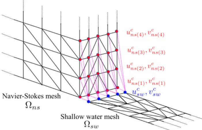
3.2 MPC for flow velocities

Let us first consider the case as illustrated in Fig.2, in which the node positions or arrangements in the FE meshes of the 2D and 3D domains, Ωsw and Ωns, conform. In this case, the flow velocities and pressures must be continuous at the interface of the two separate meshes. More specifically, regarding the nodes on the interface between the two regions, we impose the following MPC conditions (see Fig.3):

u^c_{ns (k)}=u^c_sw (k=1,· · · ,N_z^c)

v^c_{ns (k)} =v^csw (k=1,· · ·,N_z^c) (30) to ensure that the flow velocity components in the x and y directions of a certain node of Ωsw are equal to those of all the nodes of Ωns aligned in the z-direction (water depth direction) that have the same x and y coor- dinates. Here, N_z^c is the total number of the nodes on the interface belonging to Ωns that are aligned in the z- or vertical direction and therefore have the same x and y coordinates. Also, u^c_ns(k) andv^c_ns(k) represent the veloc- ity components of these nodes on the interface of Ωns,

Fig. 4 MPC condition between non-conforming meshes

whileu^c_swandv^csware the components of the average flow velocity of a certain node on the interface belonging to Ωsw.

Next, we consider the case as shown in Fig.4, in which the node positions on the interfaces belonging toΩswand Ωns do not conform with each other. Since the x and y coordinates of these nodes are different, we build the positional relationships of the nodes on the interfaces belong- ing to Ωsw and Ωns to impose the continuity conditions for the velocity components. For example, let us focus our attention to node 2 of Ωns that is located between nodes 1 and 2 of Ωsw as shown in Fig. 4. Since this node of Ωns corresponds to Point A of Ωsw, velocity component u^ns₂ can be interpolated with velocity com- ponents u^sw₁ and u^sw₂ of nodes 1 and 2 of Ωsw such that:

u^ns₂ =N₁^e(xA, yA)u^sw₁ +N₂^e(xA, yA)u^sw₂ (31) whereN₁^e(xA, yA)andN₂^e(xA, yA)are the shape functions of the line element on the interface and evaluated at coordi- natesxAand yAof Point A. This relationship is a standard MPC equation and therefore is added to the set of the 2D and 3D FE equations so that their integration can be real- ized.

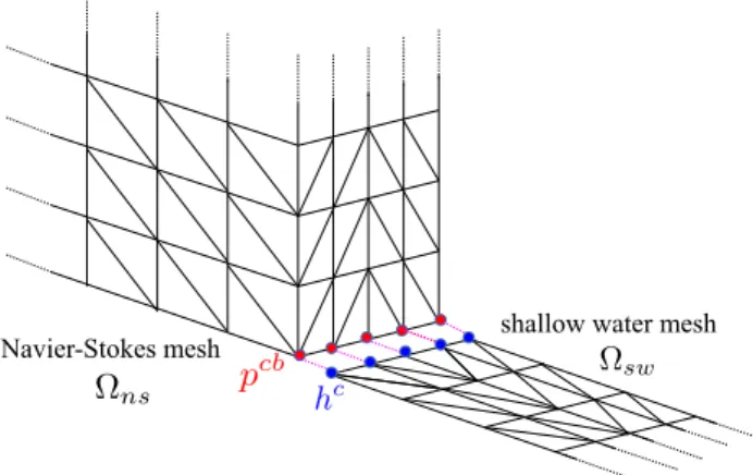
3.3 MPC for pressures

The nodal pressures on the interface ofΩns can be deter- mined according to the flow velocity, though the total water heights at the nodes on the interface belonging toΩswhave to be consistent with the pressure values at the nodes on the interface belonging to the bottom line ofΩns. Therefore, when the 2D and 3D meshes are conforming as illustrated in Fig.5, the following constraint condition is introduced:

p^cb=ρgh^c (32)

Fig. 5 MPC condition for pressure or water level

where h^c is the nodal value of the total water height in Ωsw and p^cb is the nodal value of the pressure in Ωns.

When the node arrangements are not conforming, we impose exactly the same constraint condition as in Eq. (31) on the total water heights at the nodes on the interface belonging to Ωsw and the pressure values at the nodes on the inter- face belonging to the bottom line of Ωns. Here, the water heighth^cof the 2D domain at the interface is obtained from the bottom pressure p^cb calculated in the 3D domain. The water height of the 2D domain is obtained from Eq. (31) so that the wave propagates from the 3D to 2D domains prop- erly.

3.4 Transmission method forz-component flow (vertical) velocity

In the shallow water approximation, the flow velocity is assumed to be uniformly distributed in the vertical direction and the velocity component in the z-direction,wsw, is not defined. Therefore, the velocity component in thez-direction, wns^c, on the interface belonging toΩns cannot be predeter- mined.

In order to tackle this problem, we evaluate the veloc- ity component in the z-direction,wsw, on the boundary of Ωswlocated next toΩns, based on the following free-surface kinematic condition obtained with the equation:

wsw= ∂

∂t(h+zb)+usw ∂

∂x(h+zb)+vsw ∂

∂y(h+zb) (33)

Setting the FE approximations of the flow velocity compo- nents in the x,y,z-directions and the water depth in this equation to beu^h_sw, vsw^h , wsw^h andh^h, respectively, we obtain the corresponding FE discretized equation as

Ωsw^L

ψ^hwsw^h dΩ =

Ωs^Lw

ψ^h ∂

∂t(h^h+z_b^h)

dΩ +

Ωsw^L

ψ^h

u^h_sw ∂

∂x(h^h+z^h_b)+vsw^h

∂

∂y(h^h+z^h_b)

dΩ (34)

whereψ^h is the FE approximation of the weighting func- tion ψ. Ωsw^L is the domain of elements on the interface belonging toΩsw This FE equation is solved at the same time step and its solutions, namely the nodal velocities w^hsw, are used as the data for the FE Equation (10) as the Dirichlet condition on the boundary of Ωns located next to Ωsw such that w^cns

Ωns = w^csw

Ωsw. Since spatially- constant velocity is assumed on the 3D domain side of the interface, which is equalized to that of the 2D domain side of the interface, the effects of the vertical veloc- ity cannot be considered. Then, the FE equations (10) and (16) are solved at the same time step with both this Dirichlet boundary condition and the MPC condi- tions described in the previous subsection. The solutions set of FE equations, namely the nodal velocities and total water height,u^h_sw, vsw^h andh^h, are used as the data in the right-hand side of Eq. (34) to be solved at the next time step.

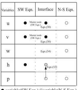
Figure6shows a relationship between variables of shal- low water equation and those of Navier–Stokes equation.

The values of the interface has been a value of the mas- ter node for MPC condition. When the flow passes though the interface from 3D domain to 2D domain, the veloci- ties in both the air part and the water part are confined by the velocity calculated from 2D shallow water equation.

Although this condition doesn’t correspond to reality per- fectly, we employ the condition for the purpose of simple calculation algorithm. This transmission method is be essen- tial to simultaneously solve the shallow-water equation and the Navier–Stokes equation. In this study, the interface is always set far away from the region in which we have to be concerned with the 3D effects so that the assumptions made for the 2D shallow water equation are valid around the interface. In this connection, the velocities of the air and the water on the 3D domain side of the interface are equal to the shallow water velocity on the 3D domain side of the interface. This indicates that the velocity distribution on the 3D domain side of the interface is uniform throughout the analysis. Strictly speaking, since this condition is phys- ically incorrect, appropriate boundary conditions should be applied. However, it is almost impossible to determine the flow velocity of the air at the interface from the 2D shallow water solution that does not provide any information about the flow in the 3D air domain. Therefore, we advocate the assumption that the effects of this setting are expected to be small.

Fig. 6 Relationship between SW Eqn. and N–S Eqn

4 Numerical examples

Three simple numerical examples are presented here to demonstrate the capability of the 2D–3D hybrid stabilized FEM proposed in this study. One of them is the solitary wave problem. This demonstrates the simple wave propagation test over a flat bed using the 2D–3D hybrid model. Second numerical example is a problem of the wave motion around a submerged breakwater. The numerical results obtained are compared with the experimental data so as to verify the accuracy of the proposed method. The last example is to demonstrate a tsunami runup analysis in an area with some structures, as a preliminary examination for the applicabil- ity of the proposed 2D–3D hybrid method to actual tsunami problems.

4.1 Solitary wave problem

In order to demonstrate the validity of the present method, we conducted a numerical analysis of the solitary wave problem.

Figure7shows the analysis model that is a water channel 120 m in length, 0.5 m in water depth and 0.05 m in width. The initial condition of the solitary wave is set at 0.05 m high.

The center region is set as the 3D Navier–Stokes domain and the other regions are the 2D shallow water domains. Figure8 shows the FE meshes for the 2D and 3D domains. The slip condition is imposed on the top, bottom and side surfaces of the water channel. The time increment was set at be 0.01s.

Figure9shows the obtained free surface profiles at different time steps. It can be seen from the result that the wave passed though the interface between the 3D and the 2D domains without any discrepancy.

Fig. 7 Analysis model for solitary wave problem

Fig. 8 FE mesh of 2D and 3D domain

Fig. 9 Numerical result of free surface profile

4.2 Wave motion around a submerged breakwater In order to verify the analysis accuracy of the proposed 2D- 3D hybrid stabilized FEM, we conduct a numerical analysis on the wave motion around a submerged breakwater [18].

Figure10shows the analysis target that is a water channel 13 m in length, 0.5 m in water depth and 0.05 m in width.

Fig. 10 Analysis model for wave motion around a submerged break- water

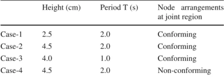
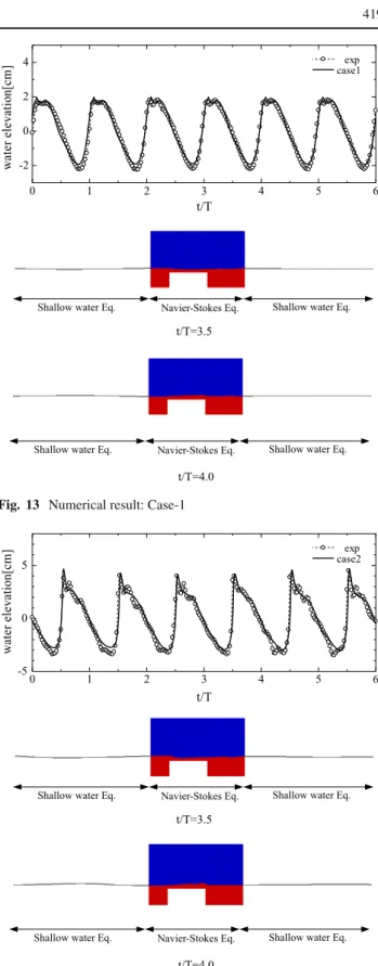
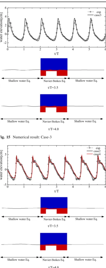
Table 1 Conditions for incident waves

Height (cm) Period T (s) Node arrangements at joint region

Case-1 2.5 2.0 Conforming

Case-2 4.5 2.0 Conforming

Case-3 4.0 1.0 Conforming

Case-4 4.5 2.0 Non-conforming

In this tank, a submerged breakwater 1.0 m in length, 0.4 m in height and 0.05 m in width is installed at a position 6 meters from the offshore. Incident waves are applied to the target from the offshore side. Only the center region around the submerged breakwater is set as the 3D Navier–Stokes domain and the other region is the 2D domain where the shallow water approximation is assumed to be valid.

Four separate conditions of incident waves are taken as shown in Table 1. Figure11shows the FE meshes for the 2D and 3D domains. Figure12shows the enlarged birds-eye view of the FE mesh at the joint region between the 2D and 3D domain for Case-4, in which the node arrangements of the 2D and 3D domains are not conforming. As shown in these figures, we prepared an unstructured mesh whose ele- ments around the submerged breakwater and the free surface become smaller as they approach its surface. For example, a minimum element length of 0.005 m is used around the free surface. The slip condition is imposed on the top, bottom and side surfaces of the water channel, while the no-slip condition is imposed on the periphery of the submerged breakwater.

The time increment used in this simulation was 0.002s, which has been determined empirically. It is to be noted that the time step required in the 3D Navier–Stokes equation must be smaller than that of the 2D shallow water equation in this calculation.

The results for Cases 1, 2, 3 and 4 are respectively pro- vided in Figs.13,14,15and16that provide the time histories of water level fluctuations measured at the center of the sub- merged breakwater in comparison with the experimental data and the profiles of the free surfaces. The origins in these

Fig. 11 FE mesh of 2D and 3D domain

Fig. 12 Enlarged birds-eye view of the FE mesh at the joint region (for Case-4)

figures are the times when the steady states are realized, respectively. As can be seen from these figures, the numeri- cal results are in agreement with the experimental ones. Also, no disturbance is observed in the profiles of the water sur- faces around both the submerged breakwater and the joint domain of the 2D–3D domains, demonstrating the stability of the proposed numerical method thanks to the performance of the stabilized FEM.

In order to confirm the capabilities of the MPC and trans- mission methods introduced in the previous section, let us focus our eyes on Cases-4, where the node arrangement does

Fig. 13 Numerical result: Case-1

Fig. 14 Numerical result: Case-2

not conform at the 2D–3D joint, and Case-2, in which the same incident wave is used. The result of Case-4 is com- pared with that of Case-2 in Fig.16, in which the two wave profiles overlap. It can be confirmed from this comparison

Fig. 15 Numerical result: Case-3

Fig. 16 Numerical result: Case-4 along with the result of Case-2

that the MPC and transmission methods implemented into the proposed 2D–3D hybrid method function properly.

In order to examine whether or not the 3D effects at the interfaces between the 2D and 3D domains are negligible in

Fig. 17 Numerical result: Case3 and Case3-w

the above numerical example, we have conducted an addi- tional numerical simulation, of which 3D analysis domain is twice as large as the original setting in the X-direction.

The interfaces of this doubled size of the 3D Navier–Stokes domain with the 2D domains are supposed to have the 3D effects at less than the original ones. We call this additional case Case-3-w and employ the same analysis condition as in Case-3, which achieves the most severe condition in terms of the Froude number. Figure17shows the time histories of water level fluctuations on the free surface measured directly above the center of the submerged breakwater in comparison with those of Case-3 and the experiment. As can be seen from this figure, the profiles of Case-3-w and Case-3 are almost the same and in agreement with the experimental result. There- fore, it seems to be safe to conclude that that the 3D effects around the interfaces are negligibly small, as the interface is set far enough away from the region where the 3D effects are considerable.

The final remark is made about the superiority in terms of the computational cost. If we generated the 3D mesh of all the analysis domain with the same fineness as that around the submerged breakwater, including 2D domain in this analysis, the number of DOF would become larger. This provisional calculation demonstrates that the proposed method enables us to simulate the offshore wave propagation and tsunami runup on a regional scale at relatively low computational cost.

Fig. 18 Analysis model for tsunami runup problem in an area involv- ing some structures

4.3 Analysis of tsunami runup with structures

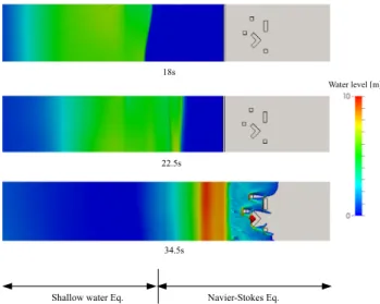
As a preliminary examination for the applicability of the proposed method to actual problems we simulate a tsunami runup involving some structures in a virtual urban area as shown in Fig.18. Here, the offshore region 400 m in length is set for the 2D shallow water equation, while the 3D Navier–

Stokes equation is solved in the remaining region with a submerged breakwater and onshore structures.

A water column with the width of 80 m and the water level of 10 m is initially located about 300 meters off the coast and is broken to generate an artificial tsunami wave.

The slip condition is imposed on the top, bottom and side surfaces and the periphery of the breakwater, while the no- slip condition is imposed on the peripheries of the submerged breakwater and buildings. A 3D unstructured mesh is gen- erated with a minimum element length of about 0.5 m in the runup area that ranges from the submerged breakwater to the region involving the buildings. Figure19shows the FE mesh around the onshore structures. The analysis with no submerged breakwater is also carried out for the sake of comparison.

Figures20and21respectively show the runup analysis results of the cases with and without the submerged break- water. It can be seen from these results that the wave for the former case spends more time than that of the latter to reach the runup area. It is thus safe to conclude that the pro- posed method can be successfully capture the effect of the submerged breakwater on the delay in the arrival time of the tsunami runup. Also, since the unstructured meshes conform-

Fig. 19 Mesh around onshore structures

Fig. 20 Numerical result of tsunami runup analysis with submerged breakwater

Fig. 21 Numerical result of tsunami runup analysis without submerged breakwater

ing to the surface configurations of the onshore structures are used, the flow regimes around the them are very sta- ble. Based on these results, it is confirmed that the proposed method is effective in simulating offshore wave propagation and tsunami runup on a regional scale involving 3D charac- teristics.

5 Conclusions

This study proposes a 2D–3D hybrid stabilized FEM to sim- ulate the offshore wave propagation and tsunami runup on a regional scale with high accuracy and at low computational costs. The 2D shallow water equation is employed for the offshore wave propagation and the 3D Navier–Stokes equa- tion is employed for the runup. The VOF method is applied to capture free-surface flows in the 3D region. To satisfy the continuity conditions for flow velocities and pressures, the standard MPC method is adopted. Also, the transmission method is introduced to approximate the vertical component of the flow velocity on the boundary of the 3D Navier–Stokes domain located next to the 2D shallow water domain. Thanks to the MPC function, the continuity conditions of flow veloc- ities and pressures at the interface can be satisfied even when unstructured meshes, which might not conform to each other, are independently generated for 2D and 3D domains.

In the numerical examples, we dealt with the problem of wave propagations around a submerged breakwater to con- firm the accuracy and stability, and the problem of a tsunami runup involving submerged and onshore structures to demon- strate the capability and effectiveness of the proposed 2D–3D hybrid method.

Acknowledgments This study is conducted with support from the Grants-in-Aid for Scientific Research (A) (Research Project No.:

25246043) “Multi-scale Numerical Experiments for Evaluation of Inter- action between Runup Tsunami and Structures”. We are grateful for the support.

References

1. Kashiyama K, Saitoh K, Behr M, Tezduyar TE (1997) Parallel finite element methods for large-scale computation of storm surges and tidal flows. Int J Numer Methods in Fluids 24:1371–1389 2. Heniche M, Secretan Y, Boudreau P, Leclerc M (2000) A two-

dimensional finite element drying-wetting shallow water model for rivers and estuaries. Adv Water Resour 23:360–371

3. Bunya S, Kubotko EJ, Westerink JJ, Dawson C (2009) Wetting and drying treatment for the Runge-Kutta discontinuous Galerkin solution to the shallow water equations. Comput Methods Appl Mech Eng 198:1548–1562

4. Takase S, Kashiyama K, Tanaka S, Tezduyar TE (2011) Space- time SUPG finite element computation of shallow-water flows with moving shorelines. Comput Mech 48:293–306

5. Yamazaki Y, Cheung KF, Kowalik Z (2011) Depth-integrated, non-hydrostatic model with grid nesting for tsunami generation, propagation, and run-up. Int J Numer Methods Fluids 67:2081–

2107

6. Guan M, Wright NG, Sleigh PA (2013) A robust 2D shallow water model for solving flow over complex topography using homoge- nous flux method. Int J Numer Methods Fluids 73:225–249 7. Aliabadi S, Abedi J, Zellars B, Bota K, Johnson A (2003) Simula-

tion technique for wave generation. Commun Numer Methods Eng 19:349–359

8. Masamura K, Fujima K, Goto C, Lida K (2000) Numerical analysis of tsunami by using 2D/3D hybrid model. J. JSCE II 54:49–61(in Japanese)

9. Masamura K, Fujima K, Goto Shigemura T (2001) Examinations of fluid forces on the structure by using 2D/3D hybrid model. Proc Hydraul Eng JSCE 45:1243–1248(in Japanese)

10. Fujima K, Masamura K, Goto C (2002) Development of the 2D/3D hybrid model for tsunami numerical simulation. Coast Eng J 44(4):373–397

11. Pringle W, Yoneyama N (2013) The application of a hybrid 2D/3D numerical tsunami inundation-propagation flow model to the 2011 off the pacific coast of Tohoku earthquake tsunami. J JSCE Ser B2 (Coastal Engineering) 69(2):I_306–I_310(in Japanese) 12. Liu GR, Quek SS (2003) The finite element method : a practical

course. Butterworth-Heinemann, Oxford

13. Brooks AN, Hughes TJR (1982) Streamline-upwind/Petrov- Galerkin formulations for convection dominated flows with par- ticular emphasis on the incompressible Navier-Stokes equations.

Comput Methods Appl Mech Eng 32:199–259

14. Tezduyar TE (1991) Stabilized finite element formulations for incompressible flow computations. Adv Appl Mech 28:1–44 15. Aliabadi S, Tezduyar TE (2000) Stabilized-finite-

element/interface-caputuring technique for parallel computation of unsteady flows with interfaces. Comput Methods Appl Mech Eng 190:243–261

16. Bova SW, Carey GF (1996) A symmetric formulation and SUPG scheme for the shallow-water equations. Adv Water Resour 19(3):123–131

17. Matsumoto J, Umetsu T, Kawahara M (2003) Stabilized bubble function method for shallow water long wave equation. Int J Comp Fluid Dyn 17:319–325

18. Sakuraba M, Kashiyama K (2003) Free surface flow using levelset method based on stablized finite element method. Proc Coast Eng JSCE 50:16–22(in Japanese)