Finite element based level set method with various reinitializations for viscous incompressible two-phase flows (Mathematical Analysis of Viscous Incompressible Fluid)

Finite element

based level

set

method with

various

reinitializations for

viscous

incompressible

two-phase

flows

Norikazu

Yamaguchi

Faculty of Human Development, University of Toyama

3190Gofuku,Toyama-shi, Toyama930-8555,Japan

Abstract. Themainobjective of the presentpaper isnumericalcomputation of

viscousincompressible two-phase flows by finite element based level set method.

A numerical resultconcerning quantitative benchmarkproblem proposed by

Hys-inget al.[11]isreported.

1.

Introduction

In this paper,

we are

concerned with numerical simulation of two-dimensional

vis-cous

incompressible and immiscible two-phase flows by finite element based level set method.

The motion ofviscous incompressible and immiscible two-phase flows is

mathe-matically formulated

as a

freeboundaryvalueproblemofthe Navier-Stokes equations.

Infreeboundaryvalueproblemsof theNavier-Stokes equations, unknown variables

are

notonlyvelocity andpressurebutalso the location of interface between two fluids. We

are

particularly interested in deformation ofthe interface and flow

near

the interface.

Thus, numericalcomputation is

one

of thereasonable waysto observethem, because

numerical computation enables

us

to

see

the development

process

ofthe motion and deformation.

Viscous incompressible two-phaseflows include various interesting phenomena in

fluid dynamics,e.g.,risingbubble,dropletimpactand dam breakingphenomena. Since there are a lot of literature concerningrising bubble problem intwo space dimension,

we

also considerrising bubbleproblem in $2D$_(however

we

do not rely

on

any

special-ties of$2D$fordiscretization oftheproblem). Inparticular,

a

numericalresultconcerning

quantitativebenchmarkproblem proposed by Hysing etal. [11] is reported.

The present

paper

is apartofjoint workwith N. Hamamuki(HokkaidoUniversity)

and K. Ohmori (University ofToyama). Details of

our

results will be published in

a

forthcomingpaper.

1.1. Governing equations

Firstofall, let

us

give

a

governing equationsof the incompressible two-phaseflows.

Let$\Omega\subset \mathbb{R}^{2}$

be

a

boundeddomainwithboundary$\partial\Omega.$ $\Omega$iscontainer of fluidsandis

assumed to be dividedintotwopartsbyinterface$\Gamma(t)$,thatis,$\Omega=\Omega_{1}(t)\cup\Gamma(t)\cup\Omega_{2}(t)$

.

Here and inwhat follows, $\Omega_{j}(t)$ is filled with fluid$j(j=1,2)$ and fluid 1 andfluid 2

fluid$j(j=1,2)$,respectively. Throughoutthepresent

paper, we

assume

that$\rho_{j}$ and$v_{j}$

are

constants $(j=1,2)$

.

Themotion offluids in$\Omega$ is govemed by the Navier-Stokes equations.

$\rho(\partial_{t}u+u\cdot\nabla u)=div(2v\mathbb{D}(u)-p\mathbb{I})+F,$ $x\in\Omega,t>0$_{, (l.la)}

$divu=0,$ $x\in\Omega,t>0$

.

_(l.lb)

The first equation (l.la) is balance of momentum and second

one

(l.lb) is equation

ofcontinuity. Here $u=(u_{1}(t,x),u_{2}(t,x))$ and_$p=p(t,x)$

are

velocity and

pressure,

respectively. They

are

unknown functions. $\rho=\rho(t,x)$ and $v=v(t,x)$

are

density and

viscosity which

are

given by

$(\rho,v)=\{\begin{array}{l}(\rho_{1},v_{1}) , x\in\Omega_{1}(t) ,(\rho_{2},v_{2}) , x\in\Omega_{2}(t) .\end{array}$ (l.lc)

Forthe density offluids,

we

assume

that$\rho_{1}>\rho_{2}$, thatis, fluid 1 is heavier than fluid2

(forexample, fluid 1 iswater and fluid2isoil

or

air). $\mathbb{D}(u)=((\partial_{j}u_{i}+\partial_{i}u_{j})/2)_{1\leq ij\leq 2}$

is thedeformationtensorand$\mathbb{I}=(\delta_{ij})_{1\leq ij\leq 2}$isthe $2\cross 2$unit matrix. 2$v\mathbb{D}(u)-p1$isthe

Cauchy stress tensorassociated withflow. $F$ denotesthebody force acting

on

fluid. In

whatfollows,

we suppose

that$F$ is gravitational force given by

$F=f_{gravity}=(0,-\rho g)$, (l.ld)

where$g$ is

a

positiveconstant whichindicates gravitational acceleration.

In addition to $u$ and $p$, location of interface $\Gamma(t)$ is also unknown in two-phase

flows. We need additional equation

on

the interface $\Gamma(t)$

.

On the interface $\Gamma(t)$, the

surface tension is taken into account. Thus, _{the interface conditions}

_on

$\Gamma(t)$

are as

follows.

$[u]|_{\Gamma(t)}=0,$ $[2v\mathbb{D}(u)-pI]|_{\Gamma(t)}\cdot n_{\Gamma(t)}=\sigma\kappa n_{\Gamma(t)}$

.

(l.le)

Here$\sigma>0$_{denotes surface}tension_constant, $K=\kappa(t,x)$isthecurvatureof theinterface

$\Gamma(t)$, and

$n_{\Gamma(t)}$ isunit normal at the interface$\Gamma(t)$ pointing into$\Omega_{1}(t)$

.

Square bracket

denotesjump of quantity

$[\bullet]_{\Gamma(t)}=\bullet|_{\Omega_{1}\cap\Gamma(t)}-\bullet|_{\Omega_{2}\cap\Gamma(t)}.$

Theinterface condition(l.le)implies thatthevelocity continuouslyacrossthe interface

$\Gamma(t)$ and surface tensionbalances thejumpof normal stress.

To observemotion of fluids in$\Omega$by

means

ofnumericalcomputation,

we

will solve

initial boundary value problem of(1.1) withinitial velocity $u(t,O)=u_{0}$, initial

inter-face $\Gamma(0)\subset\Omega$and

some

boundary condition for_$(u,p)$

on

$\partial\Omega.$

1.2. Related works andaimof thepaper

As

was

mentioned,

we

consider only rising bubble problem. Since rising bubble is

a typical phenomena of interfacial flows, there

are

much related works. Sussman,

Smereka

&

Osher [23] studiedrising bubble problem in $2D$ by finite difference based

level set method. The level set method introduced in Osher& Sethian [17] is

one

of

the standard waystocapture theinterface$\Gamma(t)$ in numerical computation of interfacial

Concerning rising bubble problem, there

are

also

a

lot of related works by finite

elementmethod, e.g.,Gross, Reichelt&Reusken[6],Tabata[24],Tornberg&Engquist

[26],Gross

&

Reusken[7] andreferences therein. Concerningrisingbubbleproblem by

finite element method, Hysing etal.[11] _proposed a quantitative benchmark problem

(see alsoDoyeuxetal. [5]). Our aim of the presentpaper is contribute the benchmark

problem proposed by Hysing etal.[11].

Aswill be seen in Section2, interface $\Gamma(t)$

can

be trackedby transportequation of

the level set function (interface is characterized by

zero

level set of level setfunction).

The level setfunction is required to have signed distance function property. However,

transport equation does not

conserve

such a property. Therefore

we

have to maintain

such

a

property in numerical computation. Theprocedure ofsigned distancefunction

maintenance is called reinitialization. There

are

various

ways

ofreinitialization, e.g.,

method based

on

partial differential equationsandfastmarchingmethod(seee.g., [7]).

We adopt reinitialization based

on

partial differential equations. In [23],

reinitial-izationbased

on

firstorderhyperbolic equation

was

introduced. Later

on

[23],Sussman

&

Fatemi [22] _proposeda modifiedversionof [23] (see also [8]). Recently,

new

reini-tialization procedures

are

proposed by Liuetal. [12] _and Basting

&

Kuzmin [1]. The

method of [1] isbased

on

nonlinearellipticpartialdifferentialequation. Thereforeitis

easy to implement the method of[1] in terms of finite element method. Inparticular,

the method of[1]

_seems

_tobe good

one

from

a

point view ofcomputational cost. We

useclassical reinitialization [23, 22] andreinitialization dueto Basting

&

Kuzmin [1] in

our

numericalcomputation (onlythelatter

case

is reported. Theformer

case

will be reported inseparatepaper).

1.3. 0rganizationof thepaper

Thispaperis organizedas follows. In Section 2 the level setmethod isintroduced. By

usingthe level set method

we

reformulate the freeboundary valueproblem of(1.1) to

be suitable form for numericalcomputation. Discretizationof reformulatedproblem is

alsogiven in Section2. InSection3reinitialization of thelevel setfunctionis discussed.

Tworeinitializations based

on

partial differential equations

are

introduced. We show

a

ournumerical resultin Section 4. We use$FreeFem++for$ourcomputation.

2.

Level

set

method and

discretization

The level set method introduced by Osher

&

Sethian [17] _is

one

of the convenient

ways to capturethe interface $\Gamma(t)$ in two-phase flows. In this section,

we

shall give

a

reformulated problem of(1.1)bythe level setmethod and give

a

discreteapproximation

ofresultantproblem.

2.1. Levelsetmethod

To capture the interface $\Gamma(t)$ in numerical computation, we

are

due to the level set

method introducedby Osher& Sethian [17]. First ofall, let

us

introduce the level set

function. Let $\phi=\phi(t,x)$ be

a

continuous scalar function defined

on

entire domain $\Omega$

and$t>0$, whose value is positivefor$x\in\Omega_{1}(t)$, negative for $x\in\Omega_{2}(t)$ and

zero

for $x\in\Gamma(t)$. Then

we

callfunction $\phi$the level set function.

A suitable choice

is

to take$\phi$equaltosigned distance function to the interface$\Gamma(t)$

.

$\phi(t,x)=\{\begin{array}{ll}dist (x,\Gamma(t)) , x\in\Omega_{1}(t) ,0, x\in\Gamma(t) ,-dist(x,\Gamma(t)) , x\in\Omega_{2}(t) .\end{array}$ (2.1)

Here dist denotes the distance function: dist$(x, \Gamma)\prime=\min_{y\in\Gamma}|x-y|$

.

Since $\phi$ is signed

distance function, $|\nabla\phi|=1$ (a.e.) must be satisfied. From (2.1), it is clear that

zero

level setof$\phi$characterizes the interface$\Gamma(t)$

.

$\Gamma(t)=\{x\in\Omega|\phi(t,x)=0\}$

.

(2.2)

When

we

choose$\phi_{0}=\phi_{0}(x)$ insuch

a

way

that$\phi_{0}$issigned distance function to the

initial interface$\Gamma(0)$, the level set.function $\phi$ is transportedby the following transport

equation:

$\frac{\partial\phi}{\partial t}+u\cdot\nabla\phi=0, t>0, x\in\Omega$_{, (2.3a)}

$\phi(0,x)=\phi_{0}(x) , x\in\Omega$

.

_(2.3b)

Since the interface$\Gamma(t)$ is represented

as

(2.2),it isenough tosolve the above transport

equation(2.3) (numerically) andinvestigatethe

zero

level setof$\phi.$

Next

we

considerareformulation of the Navier-Stokesequations (l.la). The level

setfunction $\phi$ enables

us

toreformulate $\Omega_{j}(t),\Gamma(t)$ and $(\rho,v)$

as

convenient

represen-tationfor

our

purpose.

By usingthe level set function $\phi,$ $\Omega$ and $(\rho,v)$

are

rewritten

as

follows.

$\Omega=\{\begin{array}{ll}\Omega_{1}(t) , \phi>0, \Gamma(t) , \phi=0, (\rho,v)=[Case]\Omega_{2}(t) , \phi<0; \end{array}$ (2.4)

For later

purposes, we

now

introducethe Hevisidefunction $H(\phi)$

.

$H(\phi)=\{\begin{array}{l}1, \phi\geq 0,0, \phi<0.\end{array}$ (2.5)

By using $H(\phi)$, $\rho$and $v$in (2.4)

are

rewritten

as

follows.

$\rho=\rho(\phi)=\rho_{1}H(\phi)+\rho_{2}(1-H(\phi))=\rho_{2}+(\rho_{1}-\rho_{2})H(\phi)$, (2.6)

$v=v(\phi)=v_{1}H(\phi)+v_{2}(1-H(\phi))=v_{2}+(v_{1}-v_{2})H(\phi)$

.

(2.7)

Next

we

shall give

a

level set formulation of the surface tension (l.le). By using

level set function $\phi$, the surface tension force is converted into

a

volume force ofthe

form

$f_{ST}=\sigma\kappa n_{\Gamma(t)}\delta(\phi)$

.

(2.8)

Here andinwhatfollows,$\delta(\phi)$ denotes Dirac’sdeltafunctionwhosesupport isthe

zero

level set of$\phi$

.

Furthermore, normalvector

$n_{\Gamma(t)}$ andcurvature $\kappa$

are

alsogiven by

$n_{\Gamma(t)}= \frac{\nabla\phi}{|\nabla\phi|}|_{\phi=0}$, (2.9)

Summing up the above, the resultant problem is the following system of Navier-Stokes equations and transport equation.

$\rho(\phi)(\partial_{t}u+u\cdot\nabla u)=div(2v(\phi)\mathbb{D}(u)-p\mathbb{I})+f_{ST}+f_{gravity}$, (2.11a)

$divu=0$, (2.11b)

$\partial_{t}\phi+u\cdot\nabla\phi=0$

.

(2.11c)

By thelevel setfunction,

our

aim isreducedto solve initial boundary value problem of

(2.11) with appropriateinitial data$(u,\phi)|_{t=0}$ and boundary conditions.

2.2. Discretization

Inthissubsection, weshall giveadiscretization for (2.11).

Approximation of$\delta_{\epsilon}(\phi)$ and $H_{\epsilon}(\phi)$

.

For numericalcomputationof(2.11),

we

need

some

approximations of$H(\phi)$ and$\delta(\phi)$ in terms ofcontinuousfunctions defined

over

$\Omega$

.

So, instead of_$H(\phi)$ and

$\delta(\phi)$,

we use

the following $H_{\epsilon}(\phi)$ and $\delta_{\epsilon}(\phi)$ with

some

$\epsilon>0.$

$H(\phi)\approx H_{\epsilon}(\phi)=\{\begin{array}{ll}1, \phi\geq\epsilon,\frac{1}{2}+\frac{1}{2}(\frac{\phi}{\epsilon}+\frac{1}{\pi}\sin(\frac{\pi\phi}{\epsilon})) , |\phi|<\epsilon,0, \phi\leq-\epsilon\end{array}$ (2.12)

and

$\delta(\phi)\approx\delta_{\epsilon}(\phi)=\frac{d}{d\phi}H_{\epsilon}(\phi)=\{\begin{array}{ll}\frac{1}{2\epsilon}(1+\cos(\frac{\pi\phi}{\epsilon})) , |\phi|<\epsilon,0, |\phi|\geq\epsilon.\end{array}$ (2.13)

Here $\epsilon>0$denotes thicknessof the numerical interface. Since ideal thickness of the interfaceis equalto zero, wewould like to take $\epsilon>0$ as small aspossible. However,

we

need to choose $\epsilon>0$ in such a way that $\epsilon>h$_, where $h$ denotes the mesh size

near the interface. A typical choice of$\epsilon$ is $\frac{3}{2}h$, where $h>0$indicates the mesh size

near

the $\Gamma(t)$

.

As will be

seen

in Section4,

we use

adaptive mesh refinement (AMR).

According to AMR,

we can

put

a

lot of meshpoints

near

the interface. Hence,

we can

choose $\epsilon>0$suitably small(seeFigure4.3).

Penaltymethod. Oneofthemain difficulties ofthe Navier-Stokes equations iscaused

bypressureterm$p$in(l.la) and divergencefreeconstraint(l.lb).

To relax difficulties arising from the pressure,

some

stabilization techniques are

widely usedinnumericalcomputation ofthe Navier-Stokesequations. Wehereusethe

penalty method introduced by Temam [25]. Let $\alpha>0$ be parameter ofpenalization.

Thenwe shallreplace the solenoidal condition (l.lb)by following

one.

$divu=-\alpha p$

.

(2.14)

It would be expected that $(u^{(\alpha)},p^{(\alpha)}),$which denotes solution of the Navier-Stokes

equations with (2.14), tends to genuine solution $(u,p)$

as

$\alphaarrow+0$

.

Actually, such

a limit is justified by Temam [25], Shen [20] and the author [27] _{for stationary} and

instationaryproblems.

Incontext offinite elementmethod, (2.14)changes the variational structure of the

Characteristic method. For approximation of the convection terms in the

Navier-Stokes equations (2.11a) and transport equation (2.3a),

we are

due to characteristic

method(see e.g.,Pironneau [18]).

Let $w\in \mathbb{R}^{m}(m\geq 2)$ begiven vectorfield. Then

we

consider material derivative of scalar function $\varphi$with vector$w.$

$\frac{D\varphi}{Dt}:=\frac{\partial\varphi}{\partial t}+w\cdot\nabla\varphi$

.

(2.15)

Suppose that vectorfield $X(t)\in \mathbb{R}^{m}$ defined

on

$(0,T$] solves the following ordinary

differential equations.

$\frac{dX}{dt}=w(t,X(t))$

.

(2.16)

By chain rule,

we see

that

$\frac{d\varphi}{dt}(t,X(t))=\frac{D\varphi}{Dt}$

.

(2.17)

Let $\tau>0$betime step size. Applying the backward Eulerapproximationto the left

hand side of(2.17),weobtain

$\frac{D\varphi}{Dt}=\frac{\varphi(t,X(t))-\varphi(t-\tau,X(t-\tau))}{\tau}+O(\tau)$

.

(2.18)

Set$t_{n}=n\tau(n\in N\cup\{0\})$

.

Let$x\in\Omega\subset \mathbb{R}^{m}$ bearbitrary point andlet

us

consider initial

value problem of (2.16) with initial condition $X(t_{n})=x$

.

Then the genuine solution

of such

an

initial valueproblem at$t=t_{n-1}$ is given by $X(t_{n-1})=X^{n}+O(\tau^{2})$, where

$X^{n}=x-w(t_{n},x)\tau$ isapproximatesolutionof(2.16)withtheaid ofEulermethod. By

the above arguments andTaylor’stheorem,

we

have

$\frac{D\varphi}{Dt}(t_{n},x)=\frac{\varphi(t_{n},x)-\varphi(t_{n-1},X^{n})}{\tau}+O(\tau)$

.

(2.19)

(2.19) gives

us a

first order approximation of the material derivative (2.15). Second

orderapproximation for convection-diffusion

or

Navier-Stokes equations is alsofound

in Rui

&

Tabata [19],_Notsu

_&

Tabata [13] andBen\’itez

&

Berm\’udez [2].

Semi-discretization in time. We

are

now in

a

positionto give a semi-discretization

intimefor(2.11).

Let $(u^{n},p^{n},\phi^{n})=(u^{n}(x),p^{n}(x),\phi^{n}(x))$ be approximation of $(u,p,\phi)|_{t=t_{n}}(t_{n}=$

$n\tau)$

.

Applying thecharacteristicapproximation and penalty methodto (2.11),

we

have

thefollowing semi-discretization in timefor (2.11).

$\rho_{\epsilon}(\phi^{n})\frac{u^{n+1}-u^{n}\circ X^{n}}{\tau}=div(2v_{\epsilon}(\phi^{n})\mathbb{D}(u^{n+1})-p^{n+1}\mathbb{I})+f_{ST}^{n}+f_{gravity}^{n}$_{, (2.20a)}

$divu^{n+1}+\alpha p^{n+1}=0$_{, (2.20b)}

$\underline{\phi^{n+1}-\phi^{n}x^{n}}_{=0}$

, (2.20c)

$\tau$

where$X^{n}=x-u^{n}\tau$ _and

$\rho_{\epsilon}(\phi^{n})=\rho_{2}+(\rho_{1}-\rho_{2})H_{\epsilon}(\phi^{n})$,

$v_{\epsilon}(\phi^{n})=v_{2}+(v_{1}-v_{2})H_{\epsilon}(\phi^{n})$,

$f_{ST}^{n}=\sigma K_{\epsilon}^{n}|_{\Gamma(t_{n})}\delta_{\epsilon}(\phi^{n}) , f_{gravity}^{n}=(0,-\rho_{\epsilon}(\phi^{n})g)$,

Assume that triplet $(u^{n},p^{n},\phi^{n})$ is given in (2.20). Then the systemof (2.20a) and

(2.20b) is the Stokes type systemconcerning unknownvariables $(u^{n+1},p^{n+1})$

.

Hence,

standard techniquesto solvetheStokes type system by finite element method(see.e.g,

[3], [18])

can

be applicable.

Full discretization. Finally

we

considerfulldiscretization for(2.11). Let$V_{h},\Pi_{h}$ and

$X_{h}$befinite dimensionalspaces

so

that$V_{h}\subset H^{1}(\Omega)^{2},\Pi_{h}\subset L_{0}^{2}(\Omega)$,$X_{h}\subset L^{2}(\Omega)$

.

Here

$L_{0}^{2}( \Omega)=\{p\in L^{2}(\Omega)|\int_{\Omega}pdx=0\}.$

For numerical stability,

we

choose $V_{h}\cross\Pi_{h}$

as

P2-P1 finite element space (standard

Hood-Taylorelements)and$X_{h}$

as

PI finite elementspace.

Considering variational formulation ofsemi discretizedproblem (2.20) and its

ap-proximation, we arrive at full discretization of(2.11a) and $(2.11b)$: _Find $(u_{h}^{n+1},p_{h}^{n+1})$

so

that

$\frac{1}{\tau}(\rho_{\epsilon}(\phi_{h}^{n})u_{h}^{n+1},v_{h})+(2v_{\epsilon}(\phi_{h}^{n})\mathbb{D}_{h}(u_{h}^{n+1}),\mathbb{D}_{h}(v_{h}))$

$-(p_{h}^{n+1}, div_{h}v_{h})=\frac{1}{\tau}(u_{h}^{n}\circ X^{n})+(F(\phi_{h}^{n}),v_{h})+b.d.t.$_{, (2.21a)}

$(div_{h}u_{h}^{n+1}+\alpha p_{h}^{n+1},q_{h})=0$_, (2.21b)

for any $v_{h}\in V_{h}$ and$q_{h}\in\Pi_{h}$

.

Here “b.d.$t$

.

denotes terms arising fromboundary and $)$ denotes $L^{2}$ innerproduct. For the transport equation, we do not need to consider

weakformulation. Hence by (2.20c),

we

have the followingexplicitformula.

$\phi_{h}^{n+1}=\tau\phi_{h}^{n}\circ X^{n}$

.

(2.21c)

Of

course

itis possibletoconsider weak formulation associated with(2.20c).

3. Reinitialization

Level set methodis

one

ofthesuitablemethods for numericalcomputation of interfacial

problems. In two-phaseflows, thelevel set $\phi=\phi(t,x)$ is driven by transport equation

(2.3). As

was

stated before, $\phi$mustbe

a

signed distance function (SDF), which satisfy

the Eikonal equation $|\nabla\phi|=1$ (a.e.). However, the transport equation (2.3) does not

conserve

such

a

property

even

if theinitialdata $\phi_{0}$has SDF property.

In numerical computation, $\phi_{h}^{n}$ may lose such an important property in numerical

computation

as

$n$ increases. As

a

consequence ofthis undesirablebehavior, numerical

resultwill be incorrect, if

we

donot

use

any maintenancefor level setfunction.

The procedure for recovering SDFproperty iscalled reinitialization (or

redistanc-ing). There

are

several ways ofreinitialization. In this

paper, we

consider two

reini-tialization procedures based

on

partial differential equations (PDEs). The first one is

classical procedure proposed bySussman, Smereka

&

Osher [23]. The first procedure

is based on

a

first order hyperbolic PDE. The second one is recent development by

Basting

&

Kuzmin [1]. The second procedure is based

on a

nonlinear elliptic PDE,

3.1.

Reinitializationwith hyperbolicPDE

Sussman, Smereka&Osher[23] studied incompressible two-phaseflows by finite

dif-ference based level set method. In [23], they introduced

a

reinitialization based

on

hyperbolicPDEand reportedits effectiveness by

some

numerical computations.

The reinitialization based

on

hyperbolic PDE is summarized

as

follows. Suppose

that $\phi=\phi(t,x)$ is a level set function, but it does not have SDF property $(|\nabla\phi|=1$

(a.e.)). Obtaining

some

function $\psi$

so

that $\psi$ has the

same zero

level set

as

$\phi$ and

has SDF property is objective of reinitialization. Let $\psi=\psi(s,x;t)$ be solution to the

followinginitial valueproblem.

$\frac{\partial\psi}{\partial s}=sgn(\phi)(1-|\nabla\psi|) , s>0,x\in \mathbb{R}^{2}$, (3.1a) $\psi(0,x;t)=\phi(t,x) , x\in \mathbb{R}^{2}$

_.

_(3.1b)

where $s\geq 0$indicatespseudo-time. If$\psi$ is stationary solution of(3.1a), then itwould

be expected that $\psi$ has SDF property (if such

a

stationary solution is asymptotically

stable). Hence for sufficiently large $s>0$,

_{one can use}

$\psi(s,x;t)$

as

reinitialized $\phi.$

Such

a

numericalsolution

can

be obtained by pseudotime stepping.

Since (3.1a) is first order hyperbolic partial differential equation,

we

need

some

stabilization technique for stable numerical computation. Converting (3.1a) into

con-vective form is

one

of suitable reformulations. Set $w=sgn(\phi)\nabla\psi/|\nabla\psi|$

.

Then (3.1a)

is rewritten

as

the followingequation.

$\frac{\partial\psi}{\partial s}+w\cdot\nabla\psi=sgn(\phi) , w=sgn(\phi)\frac{\nabla\psi}{|\nabla\psi|}$

.

(3.2)

Since(3.2)_isatransportequation with

source

term, stabilizationtechnique (e.g.,

char-acteristicmethodandupwind techniques)

can

be applied.

In numerical computation for initial value problem (3.2),

we

need appropriate

ap-proximationofthe sign function $sgn(\phi)$

.

Typical

ways

ofapproximations

are

sgn$( \phi)\approx sgn_{\epsilon}(\phi)=\frac{\phi}{\sqrt{\phi^{2}+\epsilon^{2}}}$

or

$\frac{\phi}{\sqrt{\phi^{2}+\epsilon^{2}|\nabla\phi|^{2}}}$ (3.3)

with parameter$\epsilon>0$_, which is

a

regularization parameter. The size of $\epsilon$ is suitably

determined by $h$ which indicates the mesh size

near

the interface. It should be noted

that $sgn(\phi)$ and $sgn_{\epsilon}(\phi)$ has the same sign. Hence the regularization (3.3) conserves

zero

level setof$\phi.$

As far

as

the authorknows, there

are no

rigorous justification that asymptotic

pro-files of(3.1)is signed distance function tothe

zero

level set of$\phi$

.

For suchaproblem,

we

have

a

mathematical result

as

follows.

Theorem 3.1. Let $d(x)$ be signeddistance

function

_{to the}

zero

_{level set}

_of

$\phi$, whose

sign is the

same

as$\phi$

.

Then therehold that the solution

of

(3.1)tendsto$d(x)$ as $sarrow\infty$

locally and uniformly in$\mathbb{R}^{2}.$

Theorem 3.1 is

a

mathematical justification of the reinitialization based

on

(3.1).

Proofis carriedoutwith theory ofviscosity solution [4]. Details will bepublished in

a

3.2. Reinitializationwith elliptic PDE

Recently Basting

&

Kuzmin[1] introduced

a

reinitialization based on energy

minimiz-ing principle. Accordminimiz-ing to Basting

&

Kuzmin [1],

_we

shall explain reinitialization

with elliptic PDE.

In context ofpurereinitialization,reinitializedlevel setfunction wouldbestationary

solutionto

an energy

minimizinggradient flow of the form

$\frac{\partial\psi}{\partial s}+\frac{\partial E}{\partial\psi}=0$, (3.4)

where $E(\psi)$ is a suitable energyfunctional and $\partial E/\partial\psi$ is the Euler-Lagrange form of

theG\^ateaux derivative. Theleast-squares solutionto the Eikonalequation $|\nabla\psi|=1$ is

defined by

$E( \psi)=\frac{1}{2}\int_{\Omega}(|\nabla\psi|-1)^{2}dx$

.

(3.5)

By using (3.5), (3.4)isreduced to thenonlinearparabolic equation

$\frac{\partial\psi}{\partial s}-div(\nabla\psi-\frac{\nabla\psi}{|\nabla\psi|})=0$

.

(3.6)

If $|\nabla\psi|>1$, then (3.6) is diffusion. On the other hand if $|\nabla\psi|<1$, then (3.6) is

anti-diffusion. (3.6)provides

us

areinitialization with parabolic PDE.If initial datais given

by original level set function $\phi$, which does not have SDF property. Then asymptotic

profile of(3.6) would be reinitialized level setfunction.

Toobtainreinitialized levelsetfunction by(3.2)or(3.6),weneedpseudo-time

step-ping. Basting

&

Kuzmin [1] proposed

a

reinitialization based

on

penalized minimizing

problem such that

$\frac{\partial E}{\partial\psi}+\frac{\partial P}{\partial\psi}=0, P(\psi;\phi)=\frac{\beta}{2}\int_{\{\phi=0\}}\psi^{2}d\sigma$ (3.7)

where $\beta\gg 1$ isparameterofpenalization. Sinceanydisplacement of the

zero

level set

would increase the valueof$P(\psi;\phi)$, the numerical solutionwill preserve theshape of

zero

level setof$\phi$for large$\beta.$

Let$\phi$be alevelset function without SDF property. A variational formulation

asso-ciated with(3.5) is given by

$((1- \frac{1}{|\nabla\psi|})\nabla\psi,\nabla\varphi)_{\Omega}+\beta\langle\psi,\varphi\rangle_{\{\phi=0\}}=0$, (3.8)

for any $\varphi\in C^{\infty}(\Omega)$

.

Since (3.8)

can

be regarded

as

a weakformulation of

a

nonlin-ear

elliptic PDE,

one

can

easily compute numerical solution to (3.8)by finite element

method. Of

courese

(3.8)isnonlinear,

we

seek numericalsolutionto(3.8)bysuccessive

approximation asfollows.

$\psi^{(0)}=\phi$_{, (3.9a)}

$( \nabla\psi^{(n+1)},\nabla\varphi)+\beta\langle\psi^{(n+1)},\varphi\rangle_{\{\phi=0\}}=(\frac{\nabla\psi^{(n)}}{|\nabla\psi^{(n)}|},\varphi) , n\geq 0$

.

(3.9b)

If $\psi^{(n)}$ is given, (3.9b)

can

be regarded

as

a weak formulation of Poisson type

equa-tion withpenalty term. One

can

obtainnumerical solution to (3.9b) by finiteelement

4.

Numerical experiments

Inthissection,

we

shall report

our

numerical result.

4.1. Quantitative benchmark problem

As

was

mentioned in Section 1,Hysingetal.[11] introduced

a

quantitative benchmark

problem of twodimensional rising bubble (precise settings of thebenchmarkproblem

will be shown). Since exact solution for rising bubble problem is notknown, it

seems

tobe worthwhile well to

compare

numerical solution with other numerical solutions by

such

a

quantitativebenchmarkproblem.

Hysingetal.[11] studiedtwotest

cases

(Case 1 and Case2)by quantitative

compar-ison between threeEuropean research groups. Two groups

are

adopted finite element

based levelset method. Later

on

[11], Doyeuxetal. [5] alsotried the

same

benchmark

problemby$Feel++$

.

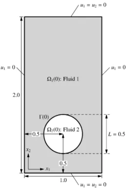
_{We also try the quantitativebenchmarkproblem.}

Figure 4.1: Initial state andboundaryconditions

Initialstateand boundary conditions. In the benchmark problem, thecontainerof

fluids is given by $\Omega=(0,1)\cross(0,2)$

.

Initially bubble $(=$fluid 2$)$ is completely

sur-rounded by fluid 1 andshape of initial bubble is circlewith radius $r_{0}(=0.25)$centered

at(0.5,0.5). Tobeprecise, initial interface is given by

$\Gamma(0)=\{(x_{1},x_{2})|(x_{1}-0.5)^{2}+(x_{2}-0.5)^{2}=r_{0}^{2}\}, r_{0}=0.25$

.

_(4.1)

For (4.1), initial level set function is signed distance function to $\Gamma(0)$, which is given

by

$\phi_{0}=\sqrt{(x_{1}-05)^{2}+(x_{2}-05)^{2}}-r_{0}^{2}$

_.

_(4.2)

Next we shall mention the boundary conditions. On the top/bottom walls of $\Omega,$

boundary condition:

$u\cdot n=0, (\mathbb{D}(u)n)-(n\cdot \mathbb{D}(u)n)=0, x\in\partial\Omega_{top/b\circ ttom}$ (4.3)

is imposed (the secondcondition is Neumann type boundary conditions for tangential

component of the normal stress). Since the unit outer normal to left/right walls is

$(\mp 1,0)$, (4.3) is reducedto$u_{1}=0.$

Figure4.1 is

a

imageof initialconfiguration of the benchmarkproblem.

Physical constants. Two dimensionlessnumbers

are

usedin risingbubble problem.

Below, $\mathcal{R}$

and $S$ denote the Reynolds number and E\"otv\"os number (Bond number),

respectively. $R$ and$S$

are

definedasfollows.

$\mathcal{R}=\frac{\rho_{1}V_{g}L}{v_{1}}, S=\frac{\rho_{1}V_{g}^{2}L}{\sigma}$

, (4.4)

where $V_{g}=\sqrt{2gr_{0}}$ is the gravitational velocity, $L=2r_{0}$ is characteristic length. The

E\"otv\"os numberindicates theratio of gravitational forces to surface tension. Table4.1

lists thephysicalconstants and dimensionlessnumbers whichspecify twotest

cases.

Table

4.1:

Physicalconstants anddimensionless numbers

Roughly speaking, the surface tension is strong in Case 1 and weak in Case 2.

Since the surface tension is strong in Case 1,

we

have to take temporal step size $\tau$

very small for numerical stability. Therefore

we

require much computational costs.

However, strong surfacetension force make shape of bubble stable. Actually, bubble

is not splitted in

our

numerical computation. On the other hand, bubble would split,

because of weak surface tension. In stability ofthe shape ofbubble, Case 2 is more

severe

thanCase 1.

Inthis

paper,

we

shall try only Case2. Ournumericalresultconcerning Case 1 will

bereportedin

a

separatedpaper.

Benchmark values. In benchmark problem ofHysing et al. [11],

some

benchmark

quantities

are

used.

Center of

mass.

Totrack the translation ofbubble, it is

common

to

use

the center

of

mass

defined

as

follows.

$X_{c}(t)=(X_{c,1}(t),X_{c,2}(t))$, $X_{\mathcal{C},i}(t)= \frac{1}{|\Omega_{2}(t)|}\int_{\Omega_{2}(t)}x_{j}dx$ $(j=1,2)$

.

(4.5)

The

mean

velocity of bubble. To observe rising speed ofbubble, the following

mean velocityof bubble isused.

$U_{c}(t)=(U_{c,1}(t),U_{c,2}(t))$, $U_{cj}(t)= \frac{1}{|\Omega_{2}(t)|}\int_{\Omega_{2}(t)}u_{j}dx$ $(j=1,2)$

.

(4.6)

$U_{c,2}(t)$ is called rise velocity. By the

use

of $U_{c,1}(t)$,

one can

investigate horizontal

symmetricityofthemotion.

Remark

4.1.

Since $1-H(\phi(t))$ is indicator function

on

$\Omega_{2}(t)$, _{$X_{cj}(t)$} and _{$U_{cj}(t)$}

$(j=1,2)$

are

computedbythe followingformulae.

$X_{cj}(t)= \int_{\Omega}(1-H(\phi))x_{j}dx/\int_{\Omega}(1-H(\phi))dx,$

$U_{c,i}(t)= \int_{\Omega}(1-H(\phi))u_{j}dx/\int_{\Omega}(1-H(\phi))dx.$

Circularity. The degreeofcircularity $\chi=\chi(t)$ is defined

as

$\chi(t)=\frac{P_{a}}{P_{b}}=\frac{Perimeterofarea-equiva1entcircle}{Perimeterofbubb1e}=\frac{\pi d_{a}(t)}{P_{b}}$

.

(4.7)

Here$P_{a}(t)$ denotes theperimeterof

a

circle with diameter_{$d_{a}(t)>0$} and such

a

circle

has

area

equaltothat ofbubble at withperimeter$P_{b}(t)$

.

By the level setfunction$\phi$andapproximation of Dirac’s delta $\delta_{\epsilon}(\phi)$, $P_{b}(t)$ is given

and approximatedby

$P_{b}(t)= \oint_{\{\emptyset=0\}}d\sigma\approx\int_{\Omega}\delta_{\epsilon}(\phi)dx$

.

(4.8)

Additional values. In addition to the above benchmark values,

we

also observe

additional two values forchecking SDFproperty ofthe level set function$\phi$ and

mass-preservation offluid2.

In order tocheck SDFproperty of$\phi$,

we

observe$L^{1}$

-mean

value$of|\nabla\phi|.$

$|| \nabla\phi(t)||:=\frac{1}{|\Omega|}\int_{\Omega}|\nabla\phi(t,x)|dx$

.

(4.9) If$\phi(t,x)$ satisfies the Eikonal equation $|\nabla\phi(t,x)|=1$ _(a.e.), then $\Vert\nabla\phi(t)||=1$ holds.

However, $||\nabla\phi(t)||=1$ does notimply $|\nabla\phi(t,x)|=1$ _(a.e.). Hence,wecall $||\nabla\phi||=1$

pseudo SDFproperty. Sinceit is hard to check SDF property foreverymeshpoints,

we

checkonly pseudoSDF property.

Ideally volume of bubble is preserved. Thus, it isimportanttochecktimeevolution

of volume ofbubble in numerical computation. VolumeofbubbleisLebesgue

measure

of$|\Omega_{2}(t)|$

.

Byusing thelevel setfunction, $|\Omega_{2}(t)|$ isgiven by

$| \Omega_{2}(t)|=\int_{\Omega_{2}(t)}dx=\int_{\Omega}(1-H(\phi))dx\approx\int_{\Omega}(1-H_{\epsilon}(\phi))dx$

.

(4.10)

4.2. Numerical experiments

In thissubsection,

we

shall show

our

numericalresult. Thecomputation

was

performed

on

Apple iMac (Late 2012)with 3.$4GHz$_{IntelCore i7}

processor

_and$32GB1600MHz$

DDR3 memory.

We

use

$FreeFem++^{1}[9$, 10$]$ for

our

numerical computation. $FreeFem++is$

a

pro-gramminglanguageand software for numerical

computation

ofpartial differential

equa-tionsby

means

of finiteelementmethod. In$FreeFem++$,there

are

variouslinearsolvers

andvariousfinite elements(fordetails,see [10]). Wesolve alinear system derived from

(2.21)by UMFPACK, whichis a sparse linearsolver. We adopted elliptic

reinitializa-tion. The maximal observation time is $T_{\max}=3.0$ and time step size ofthe following

computationis $\tau=10^{-3}.$

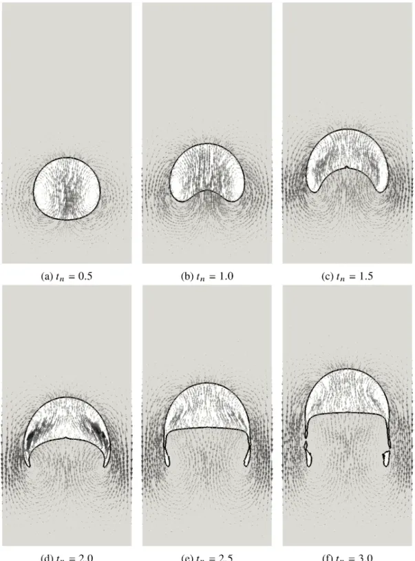
Figure 4.2 shows time evolution of

zero

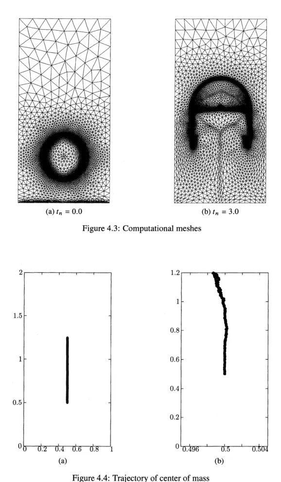
level set and velocity vector field ofour

computationand Figure 4.4shows trajectoryofcenter of

mass

$X_{c}(t_{n})$

.

We

use

adaptivemesh refinement(AMR). AMRenablesus tocapture theinterface

$\Gamma(t)$ precisely, becausewe can put muchmesh points

near

the interface. Since we use

AMR, number of triangles changes step by step. Average of number of triangles is

about 10,000and number ofverticesis about 5,000.

Figure4.3 showscomputationalmeshesat$t_{n}=0.0$(initial state)and$t_{n}=3.0$(final

state). Onecan

see

thatcomputational meshsuggeststhe shapeof interface (Fig.4.3(b)

and Fig. $4.2(f)$). Such

an

AMRtechnique is

one

ofmainfeature of

our

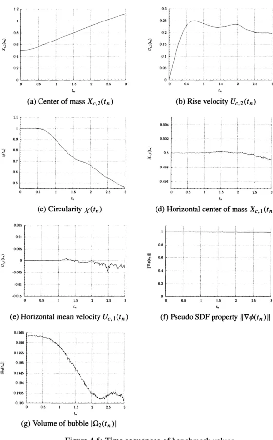
computation.

Timesequences ofBenchmark values. Figure4.5 showstime sequences of

bench-mark values.

Fig4.5(a), (b)and(c)indicatetime

sequences

ofvertical location of center of

mass

$X_{c,2}(t_{n})$, rise velocity $U_{c,2}(t_{n})$ and circularity $\chi(t_{n})$

.

Each graph is similar to

corre-sponding one in Hysing et al.[11] and Doyeux et al.[5]. In particular,

our

result is

similar to that of FreeLIFE(EPFL Lausanne) in [11].

Fig4.5(d) and (e) indicate timesequences ofhorizontal location of center of

mass

$X_{c,1}(t_{n})$ andhorizontal

mean

velocity$U_{c,1}(t_{n})$

.

These values

are

used toobservationfor

symmetricityof the rising bubble. $\overline{X_{c,1}}=0.499992787$ and$\overline{U_{c,1}}=8.75\cross 10^{-5}$, where $X_{c,1}(t_{n})$ and$\overline{U_{c,1}}$

denote timeaverageof$X_{c,1}(t_{n})$ of$U_{c,1}(t_{n})$,respectively. The

horizon-tal motion of bubble is almost symmetric, butfrom macroscopic viewsymmetricityof

themotionbreaks after$t_{n}>1.$

Fig 4.5(f) indicates time sequence of $||\nabla\phi_{h}(t_{n})||$ from macroscopic view. Time

average of$||\nabla\phi_{h}||$ is $||\nabla\phi_{h}||=0.997385$and the final value is $||\nabla\phi_{h}(3.0)||=0.993951.$

Byreinitialization,$\phi_{h}^{n}$ almostsatisfiespseudo SDF property for all$n.$

Fig4.5(g) indicatestime sequenceof the volume of fluid2. Ideally $|\Omega_{2}(t)|$ must be

conserved. However, the final valueis $|\Omega_{2}(3.0)|=0.193442$

.

Since $|\Omega_{2}(0)|=\pi r_{0}^{2}\approx$

O. 19635, 1.5% of fluid2

was

lostin

our

computation.

Acknowledgment. The author would like to

express

his sincere thanks to Professor

KatsuhiOhmori for fruitful discussion.

References

[1] C.Basting andD.Kuzmin. Aminimization-basedfinite elementformulationfor

interface-preservinglevelsetreinitialization. Computing,$95(1,$suppl.):S13-S25,2013.

[2] M. Ben\’itez andA. Berm\’udez. A second order characteristics finite element scheme for

naturalconvectionproblems. J. Comput. Appl.Math., $235(11):3270-3284$,2011.

[3] S. C. Brenner and L. R. Scott. The mathematical theory

_offinite

elementmethods,

vol-ume 15of Texts in AppliedMathematics. Springer, NewYork,thirdedition,2008.

[4] M. G. Crandall, H. Ishii, and P.-L. Lions. User’s guide toviscosity solutions of second

order partial differentialequations. Bull.Amer.Math Soc. (N.S.),$27(1):1-67$, _1992.

[5] V. Doyeux, Y. Guyot, V. Chabannes,C. Prud’homme,and M. Ismail. Simulation of

two-fluid flows using a finite element/level set method. Application to bubbles and vesicle

dynamics. J. Comput. Appl.Math.,246:251-259,2013.

[6] S. GroB, V. Reichelt,andA. Reusken. Afinite element based levelset method for

two-phaseincompressibleflows. Comput. $V\iota s$

.

Sci.,$9(4):239-257$ , 2006.

[7] S. Gross and A. Reusken. Numerical methods

_for

two-phaseincompressible flows,

vol-ume40ofSpringer Series in Computational Mathematics. Springer-Verlag,Berlin, 2011.

[8] D. Hartmann,_M.Meinke, andW.Schr\"oder. Differentialequation based constrained

reini-tializationfor level set methods. J. Comput. Phys., $227(14):6821-6845$ ,2008. [9] F.Hecht. Newdevelopmentin$freefem++$

.

_{J. Numer.}Math.,$20(3-4):251-265$ , 2012.

[10] F.Hecht. $Freefem++$

.

LaboratoireJacques-LouisLions,Universit6PierreetMarieCurie,

2015.

[11] S. Hysing, S. Turek, D. Kuzmin, N.Parolini, E. Burman, S. Ganesan, and L. Tobiska.

Quantitative benchmark computationsoftwo-dimensionalbubble dynamics. Internat. $J.$

Numer.MethodsFluids,$60(11):1259-1288$ ,2009.

[12] C. Liu, F. Dong, S. Zhu, D. Kong, and K. Liu. New variationalformulations for level

set evolution withoutreinitialization with applications to image segmentation. J. Math

Imaging Vsion,41(3):194-209,2011.

[13] H. Notsu and M. Tabata. A single-step characteristic-curve finite element scheme of

second order in time for the incompressible Navier-Stokes equations. J. Sci. Comput.,

38(1):1-14,2009.

[14] K. Ohmoriand N. Yamaguchi. in preparation.

[15] _{K. Ohmori and N. Yamaguchi. Visualization of nonlinear phenomena with} $FreeFem++$

andparaview: Application to reaction-diffusion system and fluid dynamics. $Mem.$ $Fac.$

Human.Devel. Univ. Toyama.,$9(1):221-241$ , 2014(in Japanese).

[16] _K. Ohmori, N. Yamaguchi, N. Hamamuki, and F. Hecht. Numerical investigation of

two-fluid flows by$FreeFem++and$themathematicalvalidation of thereinitialization. $in$

preparation.

[17] _{S. Osher and} J. A. Sethian. Fronts propagating withcurvature-dependent speed:

algo-rithmsbasedonHamilton-Jacobi formulations. J. Comput. Phys.,$79(1):12A9$, 1988.

[18] _{O. Pironneau. Finiteelementmethods}

_{for fluids.}

_{John Wiley &Sons Ltd., Chichester,} 1989.

[19] H.Rui and M. Tabata. A second ordercharacteristicfinite element scheme for

[20] J. Shen. Onerrorestimates ofthe penaltymethod for unsteady Navier-Stokes equations.

SIAM J. Numer.Anal.,$32(2):386-403$, 1995.

[21] R. S.Strichartz. A guide todistribution theory andFourier

_transforms.

World Scientific

Publishing Co.Inc., RiverEdge,NJ,2003.

[22] _{M. Sussman and E. Fatemi. An}efficient,interface-preserving level set redistancing

algo-rithm andits applicationto interfacial incompressible fluid flow. SIAMJ. Sci. Comput.,

20(4):1165-1191 (electronic), 1999.

[23] M. Sussman,P. Smereka, andS. Osher. A levelsetapproach forcomputingsolutions to

incompressible two-phase flow. J. Comput. Phys., 114:146-159, 1994.

[24] M. Tabata. Finite element schemes based on energy-stable approximation fortwo-fluid

flowproblems with surfacetension. HokkaidoMath. J., $36(4):875-890$,2007.

[25] R. Temam. Unem\’ethoded’approximationde lasolutiondes \’equations de Navier-Stokes.

Bull. Soc.Math. France,96:115-152, 1968.

[26] A.-K.Tomberg and B. Engquist. Afinite elementbasedlevel-set method formultiphase

flowapplications. Comput. $Vs$

.

_{Sci.,$3(1-2):93-101$,}2000.

[27] N. Yamaguchi. Mathematicaljustification ofthepenalty method forviscous

(a)$t_{n}=0.5$ (b)$t_{n}=1.0$ (C)$t_{n}=1.5$

(d)$t_{n}=2.0$ ($e$)$t_{n}=2.5$ $(t\gamma t_{n}=3.0$

Figure 4.2: Time evolution of the

zero

level set of $\phi_{h}(t_{n})$ and velocity vector fields.

(a)$t_{n}=0.0$ (b)$t_{n}=3.0$

Figure 4.3: Computational meshes

(a) (b)

$\ell_{h},$

$\ell_{h},$ $\ell_{n}$

(a)Center ofmass$X_{c,2}(t_{n})$ (b)Rise velocity$U_{c,2}(t_{n})$

$\overline{\vee s\vee}$ $\hat{\frac{s}{\dot{\aleph}^{-}}}$

05 15

$25 05 1B 25$

$t_{\eta}$ $l_{n}$

(c)Circularity$\chi(t_{n})$ (d)Horizontalcenterofmass$X_{c,1}(t_{n})$

$\overline{\frac{\prime_{arrow}\prime}{\dot{b}arrow}}$

$t_{n}$

(e) Horizontalmeanvelocity$U_{c,1}(t_{n})$ (f)Pseudo SDF property $||\nabla\phi(t_{n})||$

$\underline{\overline{\hat{\check{c^{\aleph}}\sim^{l}}}}$

(g)Volume ofbubble $|\Omega_{2}(t_{n})|$