Scene Adaptive Exposure Time Control for Imaging and Apparent Motion Sensor

(1)

LETTER

Special Section on Image Media Quality

Scene Adaptive Exposure Time Control for Imaging and Apparent Motion Sensor

Misaki SHIKAKURA^†a),Nonmember, Yusuke KAMEDA^†b),andTakayuki HAMAMOTO^†c),Senior Members

SUMMARY This paper reports the evolution and application potential of image sensors with high-speed brightness gradient sensors. We propose an adaptive exposure time control method using the apparent motion estimated by this sensor, and evaluate results for the change in illuminance and global/local motion.

key words: image sensor, exposure time control, apparent motion sensor, moving object

1. Introduction

CMOS image sensors have been developed for surveillance and industrial equipment cameras. In these applications, it is important to capture images with clear details for image recognition and object tracking. Since the exposure param- eters (including exposure time, which is examined in this paper) are not appropriate, overexposure and underexposure may occur when the illuminance varies with artificial or nat- ural light. Therefore, it is necessary to capture an image with the exposure time that is adjusted to the illuminance level of the scene. At the same time, motion blur must be suppressed when the camera or subject is moving.

Many auto exposure algorithms adopt the average brightness value of the scene to control the exposure time.

The method based on the brightness value in[1]adjust the exposure time for the important object such as a moving object. The weight of the segmented moving object is higher through object tracking, and control the proper exposure time for moving objects. However, this approach probably cause motion blur When the moving subject is dark and exposure time is set long.

Imaging with a short exposure time can suppress motion blur, and the exposure time can be estimated by using motion estimation. High frame rate imaging is effective for improving the accuracy of motion estimation[2],[3]. The correlation between frames at high frame rate is so high that the computational complexity of motion estimation is re- duced. However, many frames are needed to output from the image sensor to a signal processing circuit outside the sensor, and imaging at high frame rate increases the data rate.

Several methods[4]–[7]mount a simple processing circuit Manuscript received June 30, 2020.

Manuscript revised October 18, 2020.

Manuscript publicized January 7, 2021.

†The authors are with the Graduate School of Engineering, Tokyo University of Science, Tokyo, 125-8585 Japan.

a) E-mail: [email protected] b) E-mail: [email protected] c) E-mail: [email protected]

DOI: 10.1587/transfun.2020IML0007

for estimating motion on the sensor. Since it is unnecessary to output many frames from the sensor, motion estimation can be performed without excessively increasing the data rate and motion estimation can be performed in real time.

Nose et al.[4]estimate the motion by extracting the moving subject by the background subtraction method, and obtain- ing the displacement of the center of gravity of the moving subject between frames. They assume that the background is fixed and therefore this method is not effective when the camera or multiple subjects move.

In order to calculate motion vector for each pixel with high accuracy, we developed an image sensor that has two types of pixels, one type for acquiring images and the other type for estimating motion[7]. It can estimate apparent motion while acquiring an image. Motion estimation uses a photodiode voltage that outputs non-destructively over very short time intervals like high frame rate imaging. After the motion estimation is complete, a sufficiently accumulated voltage is read out so that it is possible to acquire an image with a high signal-to-noise ratio (SNR).

In this paper, we propose a method for controlling exposure time for this image sensor by apparent motion [8].

Whether or not there is a moving subject is determined based on the result of apparent motion. In static scenes there is no moving object, exposure time is adjusted according to the mean brightness value. In dynamic scenes, it is adjusted the longest exposure time that makes moving objects appear motionless using apparent motion.

2. Image Sensor with Apparent Motion Estimation The image sensor [7] can estimate apparent motion while acquiring an image. The architecture of the image sensor and timing of reading start are shown in Figs. 1 and 2. The image sensor has two types of pixels, one type for acquiring images and the other type for estimating motion. The pixels for motion estimation are arranged in 2×2 cells. In cell numbers 1, 2, and 3, the voltage of the photodiode is read out non-destructively over very short time intervals, and apparent motion is estimated by the temporal variation in the voltage. After the motion estimation, the voltage of a photodiode with sufficient stored charge is read out in the pixels and cell number 4. Each readout timing is controlled by a pixel/cell selector. Because the pixels and the cells have photodiodes of different sizes, light sensitivity correction is performed outside the sensor.

Motion estimation based on the gradient method was Copyright c2021 The Institute of Electronics, Information and Communication Engineers

(2)

Fig. 1 Architecture of the image sensor with apparent motion estimation [8]. The sensor consists of pixels and 2×2 cells. White cells and pixels are used for imaging, and black cells are used for motion estimation.

Fig. 2 Timing of reading start. The cell can be read out multiple times over short time intervalTduring pixel exposure periodτ.

performed using temporal variation of the voltage in the 2×2 cells. Spatial and temporal gradients were calculated in the analog domain, and motion vectors were estimated on the FPGA (Field Programmable Gate Array) using these gradients. We show how to calculate the spatial and temporal gradients in Fig. 3. A frame that is read out at intervals of T seconds in cells is called a sub-frame. The time variation∆V_PDn(k) of the photodiode (negative) voltageV_PDn(k) in cellnat sub-framekis

∆VPDn(k)=VPDn(k−1)−VPDn(k) (1) and corresponds to the predicted value of illuminance. The spatiotemporal gradientI_x(k),I_y(k), andI_t(k) are:

Ix(k) = ∆VPD2(k)−∆VPD1(k), (2) Iy(k) = ∆VPD3(k)−∆VPD1(k), (3) It(k) = ∆VPD1(k+1)−∆VPD1(k). (4) Assuming that the speed of the motion between sub-frames is constant and that the motion vector is sufficiently small, the constraint equation[9]for the gradient method is:

Ix(k)u(k)+Iy(k)v(k)=−It(k) (5) whereu andvare horizontal and vertical velocity vectors

Fig. 3 Spatial and temporal gradients on cells. Ix(k) andIy(k) are the spatial gradients andI_t(k) is the temporal gradient.

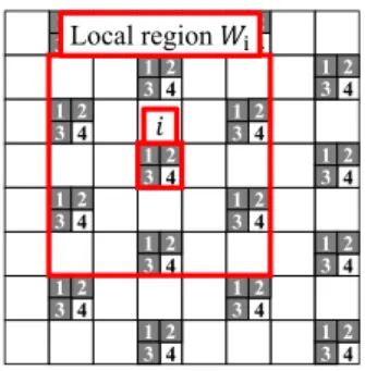
Fig. 4 Local regionWi for motion estimation based on Lucas-Kanade method[9]. W_i which is centered on the pixel of interestiincludes the neighborhood of six cells.

representing the number of pixels traversed between sub- frames. The vectors are then uniquely estimated using the Lucas–Kanade method [9], which assumes the neighborhood of the pixel of interest also has the same motion vectors. Figure 4 shows the local region Wi centered on the pixel of interesti. The motion vectorsu_iandv_iat pixel posi- tioniare estimated by the least-squares method by the spatial and temporal gradient as

"

ui

v_i

#

=−

" P

∈WiI_x² P

∈WiIxIy

P

∈W_iI_xI_y P

∈W_iI_y²

#−1" P

∈W_iIxIt

P

∈W_iIyIt

# . (6) To reduce noise, letA(t) be the average motion vector of the sub-frame sequence in frametand it is given as

A(t)= 1 M

1 N

M

X

k=1 N

X

i=1

"

ui(k) v_i(k)

#

(7) whereNis the number of the pixel of interest, andMis the total number of sub-frames in a single frame.

3. Adaptive Exposure Time Control

We controlled exposure time for illuminance and motion of the scene using the apparent motion estimated by the sensor. First, static and dynamic scenes were differentiated by apparent motion. Next, in static scenes, the exposure time was adjusted according to the mean brightness value, while in dynamic scenes, the exposure time was adjusted according to the apparent motion.

(3)

In a static scene withkA(t−1)k < α(αthreshold of magnitude), the camera and subject are static, and the illuminance changes between frames. Exposure time is controlled based on the mean brightness value in the method [10]. Letτ(t) be the exposure time at frame t. The mean brightness value at frametispt, and the exposure timeτis adjusted according to the previous frame:

τ(t)=τ(t−1)× p_m pt−1

(8) wherepmrepresents the mid-tone value. If the illuminance changes between frames, an exposure time adjusted according to the previous frame is not appropriate. The absolute errorDis given as

Dt=|pm−pt| (9)

To compensate the image with the adjusted exposure time, the previous and current frames are fused with the weight given in Eq. (11). D is used as the weight for the other frame so that the frame with the smaller error has the higher weight.Ytis the output image.

Y_t=(

X_t^τ i fθ1<p_t< θ2

X_t^comp otherwise (10)

X_t^comp= DtX_t−1^τ +Dt−1X_t^τ Dt−1+Dt

(11) whereθ₁ andθ₂ are the thresholds of the appropriate mean brightness value (θ1 < pm < θ2), andX_t^τis the image captured with the adjusted exposure timeτ.

In a dynamic scene withkA(t−1)k = α, we assume that the camera or subject is moving. The exposure time is adjusted to suppress motion blur by using the magnitude:

τ(t)= T

kA(t−1)k (12)

4. Evaluation by Simulation

We simulated adjusting the exposure time for both static and dynamic scenes. The cell readout interval T was set to 1/1600 sec, and M, which is the total number of sub- frames in a single frame, was set to 8. The exposure time is within 1/1600–1/200 sec with an interval of 1/1600 sec. To simulate the motion estimation, we reproduced 8-bit intermediate images during exposure period and added random noise with a standard deviation 3 to these images. In the simulation, we assumed that noise was constant regardless of brightness and shot noise was not considered. The intermediate images were 512×512 pixels, and one pixel of the intermediate image corresponded to one cell in Fig. 1.

The motion estimation was calculated using the brightness gradients of the intermediate images. The acquired image were the intermediate image scaled down to 256×256 pixels by the area average method, however, in the 2×2 cell,

Fig. 5 ImagesX_t^1/200captured at the longest exposure time 1/200 sec at frametwhen exposure time is not adjusted. The illuminance changes every two frames.

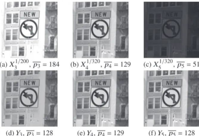
Fig. 6 Imaging results after exposure time adjustment and compensa- tion. ImagesX^τ_t captured with adjusted exposure timeτ(top), the output imagesY_t(bottom) at framet, and the mean brightness valuep. Thepof the output images was approximately the mid-tone valuepm=128.

the brightness value of only the 4th cell was extracted because the pixels for calculating the motion vector (cells 1–4) have a different light sensitivity from the other pixels. The threshold of magnitudeαwas 0.1, which corresponds to an average motion of 0.1 pixel per sub-frame. The mid-tone valuepmwas 128 and thresholdsθ1andθ2were 78 and 179, respectively. In this motion estimation method, the local re- gionWiincluded seven block cells, as shown in Fig. 4. The number of the pixel of interestNwas set to 128×128.

In a static scene, we evaluated the adjusted exposure time based on the mean brightness value when the illuminance changed every two frames. Figure 5 shows images captured with the longest exposure time, 1/200 sec, at each frame. Figure 6 shows images captured with the adjusted exposure time, the output images, and the mean brightness value p. Att =4 with no change in the illuminance,p4is approximately 128 as shown in Fig. 6(b). That means the exposure time control is appropriate. Fort = 3, andt = 5 with the illuminance change, the difference between pand 128 is large as shown in Figs. 6(a) and (c). Thus, the exposure time control is not appropriate. However, as shown in Figs. 6(d) and (f), both p₃ and p₅ of the output images are approximately 128. Therefore, these results showed that we could properly control the exposure time and compensate the brightness in a static scene with changing the illuminance. In terms of detail, the output image in Fig. 6(d) lost the detail in the lower right region. The reason for the loss of detail was that the weight of Fig. 6(a), which was

(4)

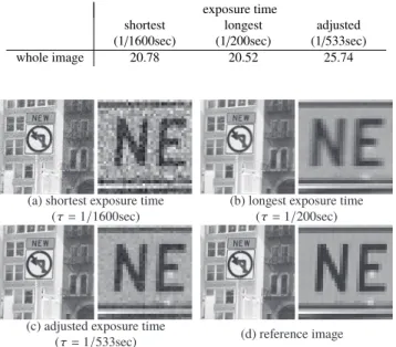
Table 1 PSNR (dB) comparison for images captured with the different exposure time when the camera is moving.

exposure time shortest

(1/1600sec)

longest (1/200sec)

adjusted (1/533sec)

whole image 20.78 20.52 25.74

Fig. 7 Comparison of images captured with different exposure timeτ when the camera is moving. (c) contains less noise than (a), and less motion blur than (b).

overexposed in the lower right region, was high when fus- ing according to Eq. (11).

In dynamic scenes, we evaluated the quality of images captured with the adjusted exposure time when the camera or subject moves 0.8 pixels in 1/1600 sec. To simulate the proposed method, we added motion blur to the images. We simulated in the two type of the scenes, where the camera moved as shown in Fig. 7 and where the train moved as shown in Fig. 8. Figures 7(a)–(c) and 8(a)–(c) show images captured with the shortest, the longest, and the adjusted exposure time. Figures 7(d) and 8(d) show the reference image with noiseless and motionless. We corrected these images to the same brightness using the ratio of exposure time.

The PSNR values are shown in Tables 1 and 2. In Figs. 7(a) and (c), the adjusted exposure time is longer than the shortest exposure time. As a result, the amount of noise with the adjusted exposure time is less. Also, in Figs. 7(b) and (c), the displacement at the long exposure time is 6.4 px, while that at the adjusted exposure time is 2.4 px. Thus, the image with the adjusted exposure time has less motion blur.

In Table 1, the PSNR of the image with the adjusted exposure time is the highest. Likewise, the adjusted exposure time image has clear details in Fig. 8. In Table 2, although the PSNR of the image with the adjusted and the longest exposure time is almost same value, the adjusted exposure time image is highest quality in the moving area. The main reason is that the displacement at long exposure is 6.4 px, while the displacement at adjusted exposure time is 3.2 px, which suppresses motion blur. According to these results, we were able to control the exposure time that was adaptive to motion.

Table 2 PSNR (dB) comparison for images captured with the different exposure time when the train is moving.

exposure time shortest

(1/1600sec)

longest (1/200sec)

adjusted (1/400sec)

whole image 20.48 29.84 29.70

moving area 19.86 19.93 21.94

Fig. 8 Comparison of images captured with different exposure timeτ when the train is moving. (c) contains less noise than (a), and less motion blur than (b).

5. Conclusion and Future Works

To improve the image quality in terms of exposure time of an image sensor with motion estimation function, we proposed a method to control exposure time to adjust to illuminance and motion. In static scenes, we controlled the exposure time using the mean brightness value, and obtained images with an appropriate brightness level. In dynamic scenes, we used motion to control the exposure time, and obtained images with less noise and less motion blur. We evaluated the effectiveness of the proposed method by simulation. The proposed method was able to capture images with clear details, which are useful for image recognition and object tracking.

In the future, we will consider reconstruction processing that improves image quality not only in moving subjects but also in static areas. In addition, we will further improve the accuracy of exposure time control by focusing on the motion vector only in the local region when there is local motion. We will also verify the proposed method in a dark scene since it is assumed that shot noise reduce the accuracy of motion estimation and affect exposure time control.

Acknowledgments

This work was supported by JSPS KAKENHI Grant Num- bers JP17K12717 and JP20K19829.

References

[1] W. Kao, “Real-time image fusion and adaptive exposure control for

(5)

smart surveillance systems,” Electron. Lett., vol.43, no.18, pp.975–

976, 2007.

[2] H. Katayama, D. Sugai, and T. Hamamoto, “High-accuracy motion estimation by variable gradient method using high frame-rate images,” IEICE Trans. Fundamentals, vol.E95-A, no.8, pp.1302–1305, Aug. 2012.

[3] T. Komuro, Y. Watanabe, M. Ishikawa, and T. Narabu, “High-S/N imaging of a moving object using a high-frame-rate camera,” 2008 15th IEEE International Conference on Image Processing, pp.517–

520, 2008.

[4] A. Nose, T. Yamazaki, H. Katayama, S. Uehara, M. Kobayashi, S. Shida, M. Odahara, K. Takamiya, S. Matsumoto, L. Miyashita, Y. Watanabe, T. Izawa, Y. Muramatsu, Y. Nitta, and M. Ishikawa,

“Design and performance of a 1 ms high-speed vision chip with 3D-stacked 140 GOPS column-parallel PEs,” Sensors (Switzerland), vol.18, no.5, May 2018.

[5] T. Otaka, T. Hiraga, and T. Hamamoto, “Current-mode frame subtraction circuit for onsensor object tracking,” ISPACS 2009 - 2009 International Symposium on Intelligent Signal Processing and Com- munication Systems, Proceedings, pp.505–508, 2009.

[6] Y. Kawashima, K. Nakayama, T. Hamamoto, and K. Kodama,

“High-speed-computational image sensor for detection of 2D motion vector by using single pixel matching,” 2010 IEEE Interna- tional Conference on Multimedia and Expo, ICME 2010, pp.872–

877, 2010.

[7] T. Aratani and T. Hamamoto, “A 4-cell per pixel structure image sensor with gradient-based motion estimation function,” IEICE Techni- cal Report, vol.118, no.338, pp.49–52, 2018.

[8] M. Shikakura, Y. Kameda, and T. Hamamoto, “Adaptive exposure time control for image sensor estimating motion distribution,” Tenth International Workshop on Image Media Quality and its Applica- tions, IMQA2020, pp.37–40, 2020.

[9] B. Lucas and T. Kanade, “An iterative image registration technique with an application to stereo vision,” 7th international joint conference on Artificial Intelligence, pp.674–679, 1981.

[10] Q. Gu, A. Al Noman, T. Aoyama, T. Takaki, and I. Ishii, “A high- frame-rate vision system with automatic exposure control,” IEICE Trans. Inf. & Syst., vol.E97-D, no.4, pp.936–950, April 2014.