Tactile Information Processing by Distributed-Type Tri-axial Force Sensor for Robot Finger

(1)

Tactile Information Processing by Distributed-Type Tri-axial Force Sensor for Robot Finger

Akihito I

TO*

, Nobutaka T

SUJIUCHI**

, Takayuki K

OIZUMI***

and Hiroko O

SHIMA****

(Received July 20, 2007)

To realize advanced manipulation, it is necessary to acquire forces and moments applied to the fingertips of the robot hand.

Moreover, it is vital to evaluate the slip between the contacted object and the sensor. Thus, the force applying to the fingertips of the robot hand needs to be measured as distribution information of forces in three directions. Until now, we have developed a distributed-type tri-axial force sensor with 12 sensor elements that can detect vertical force and shear force. The elements are arranged on a 15 mm u 20 mm area on the same plane. In the present paper, tactile information processing algorithms to measure applied force and moment and to evaluate slip, using this developed sensor, is developed. The experimental results demonstrated the effectiveness of these tactile information processing algorithms.

-G[YQTFU force sensor, tactile information processing, robot finger, strain gauges, distributed-type tactile sensor

ࠠ࡯ࡢ࡯࠼ജ࠮ࡦࠨ㧘⸅ⷡᖱႎಣℂ㧘ࡠࡏ࠶࠻ᜰ㧘ᱡࠥ࡯ࠫ㧘ಽᏓဳ⸅ⷡ࠮ࡦࠨ

ࡠࡏ࠶࠻ᜰߩߚ߼ߩಽᏓဳਃゲജ࠮ࡦࠨࠍ↪޿ߚ⸅ⷡᖱႎಣℂ

દ⮮ᓆੱ㧘ㄞౝિᅢ㧘ዊᴰቁਯ㧘ᄢፉ⵨ሶ

㧚 ߪߓ߼ߦ

⃻࿷㧘ࡠࡏ࠶࠻ߦߪ㧘Ꮏᬺߩߺߥࠄߕ㧘㜞ᐲߥ૞

ᬺࠍⴕ߁੺⼔࡮⑔␩ᯏེߥߤߦᵴべߩ႐߇ᐢ߇ࠆߎ ߣ߇ᦼᓙߐࠇߡ޿ࠆ^{1, 2)}㧚ߎࠇߦ઻޿㧘ࡠࡏ࠶࠻ࡂࡦ

࠼ߢ‛૕ࠍེ↪ߦᛠᜬߒߚࠅᠲ૞ߒߚࠅߔࠆ⎇ⓥߥ ߤ߇ⴕࠊࠇߡ߈ߚ ³⁾㧚ߒ߆ߒ㧘ੱ߇஻߃ࠆޟེ↪ߥ ᚻޠߦᲧߴࡠࡏ࠶࠻ࡂࡦ࠼ߩེ↪ߐߪ࿶ୟ⊛ߦഠࠆ

ߣ⸒ࠊߑࠆࠍᓧߥ޿㧚ߎࠇߪ㧘ੱ߇஻߃ࠆޟེ↪ߥ ᚻޠߪఝࠇߚࠕࠢ࠴ࡘࠛ࡯࠲ߢ޽ࠆߩߣหᤨߦ㧘࿶

ⷡ㧘ജⷡ㧘᷷ⷡ㧘಄ⷡ㧘∩ⷡ㧘ᒢᕈ․ᕈ⹺⼂㧘⴫㕙 ᒻ⁁⹺⼂ߥߤࠍ㜞ᗵᐲߢ࠮ࡦࠪࡦࠣߔࠆߎߣ߇ߢ߈ ࠆఝࠇߚ⸅ⷡ࠮ࡦࠪࡦࠣ⢻ജࠍᜬߞߡ޿ࠆߩߦኻߒ㧘 ࡠࡏ࠶࠻ࡂࡦ࠼ߦ៞タߒߡ޿ࠆ⸅ⷡ࠮ࡦࠨߩ࠮ࡦࠪ

ࡦࠣ⢻ജ߇චಽߢߥ޿ߚ߼ߢ޽ࠆ^{4, 5)}㧚ᣢሽߩ⸅ⷡ࠮

* Department of Mechanical Engineering, Doshisha University, Kyoto, JSPS Research Fellow Telephone: +81-774-65-6974, Fax: +81-774-65-6488, E-mail: [email protected]

** Department of Mechanical Engineering, Doshisha University, Kyoto Telephone/Fax: +81-774-65-6493, E-mail: ntsujiuc @mail.doshisha.ac.jp

*** Department of Mechanical Engineering, Doshisha University, Kyoto Telephone/Fax: +81-774-65-6492, E-mail: tkoizumi @mail.doshisha.ac.jp

**** Department of Mechanical Engineering, Doshisha University, Kyoto Telephone/Fax: +81-774-65-6488, E-mail: kt070033 @mail.doshisha.ac.jp

(2)

ࡦࠨߪ㧘㕒㔚ኈ㊂ဳ㧘ࡇࠛ࠱ᛶ᛫ဳ㧘శቇဳ㧘ᱡࠥ

࡯ࠫဳߥߤ⒳ޘߩᣇᴺ ^6-10)߇޽ࠆ߇㧘޿ߕࠇ߽࿶ജ ߩߺࠍᬌ಴ߔࠆනᯏ⢻ߢ޽ࠆ႐ว߇ᄙ޿⁵⁾㧚߹ߚ㧘

3

ゲ߽ߒߊߪ

6

ゲജ࠮ࡦࠨߢ޽ࠆ႐วߢ߽㧘ዊဳൻ߇

࿑ࠄࠇߡ߅ࠄߕ㧘ࡠࡏ࠶࠻ࡂࡦ࠼ߩᜰవߦⶄᢙ୘៞

タߔࠆߎߣߪߢ߈ߥ޿㧚ᓥߞߡ㧘ജⷡߦߩߺᵈ⋡ߒ ߡ߽ജߩ૞↪ὐࠍᱜ⏕ߦ⸘᷹ߔࠆߎߣ߇ߢ߈ߥ޿㧚 ߎࠇߦࠃࠅࡠࡏ࠶࠻ࡂࡦ࠼ߦࠃࠆᠲࠅߥߤߪ⺋Ꮕߦ ᒙ޿߽ߩߦߥߞߡߒ߹޿㧘೙⚂᧦ઙ߇ᄙᢙ⊒↢ߒߡ ߒ߹߁㧚ߘߎߢ㧘ᚒޘߪ㧘ޟེ↪ߥᚻޠߩታ⃻ߦ․ߦ

㊀ⷐߢ޽ࠆធ⸅ജ㧘ធ⸅૏⟎㧘Ṗࠅ߇ᬌ಴น⢻ߥ⸅

ⷡ࠮ࡦࠨࠍ㐿⊒ߒߡ޿ࠆ㧚ᧄ⸅ⷡ࠮ࡦࠨߪ㧘ု⋥ജ ߣߖࠎᢿജࠍ⸘᷹ߢ߈ࠆ࠮ࡦࠨ⚛ሶࠍᄙᢙ㈩೉ߒߚ ಽᏓဳਃゲജ࠮ࡦࠨߢ޽ࠆ㧚ᧄ࠮ࡦࠨߪ㧘ਃಽജߩ ಽᏓᖱႎࠍᓧࠆߎߣ߇น⢻ߢ޽ࠆߚ߼㧘ᓥ᧪ߩ⸅ⷡ

࠮ࡦࠨߦᲧߴធ⸅⁁ᘒߦߟ޿ߡߩࠃࠅᄙߊߩᖱႎࠍ ᓧࠆߎߣ߇ߢ߈㧘ᓥ᧪ߩ⸅ⷡ࠮ࡦࠨߢߪ⸘᷹ߢ߈ߥ ߆ߞߚ⸅ⷡᖱႎࠍᓧࠆߎߣࠍน⢻ߦߔࠆߣ੍ᗐߐࠇ ࠆ㧚

ᧄ⎇ⓥߢߪ㧘ޟེ↪ߥᚻޠߩታ⃻ߦ․ߦ㊀ⷐߥ⸅ⷡ

ᖱႎߢ޽ࠆ࠮ࡦࠨߦ૞↪ߔࠆജ㧘ࡕ࡯ࡔࡦ࠻ߩ⸘᷹㧘

෸߮㧘Ṗࠅߩᬌ಴߇น⢻ߥ⸅ⷡᖱႎಣℂࠕ࡞ࠧ࡝࠭

ࡓߩ㐿⊒ࠍ⋡⊛ߣߔࠆ㧚ᧄ⺰ᢥߢߪ㧘㐿⊒ߒߚࡠࡏ

࠶࠻ᜰ↪ಽᏓဳਃゲജ࠮ࡦࠨߩ

5

୚ࡕ࠺࡞ࠍ↪޿ߡ㧘

⸅ⷡᖱႎಣℂࠕ࡞ࠧ࡝࠭ࡓߩ᦭ലᕈߩᬌ⸽ࠍⴕ߁㧚

㧚 ಽᏓဳਃゲജ࠮ࡦࠨ

ᧄ┨ߢߪ㧘⹜૞ߒߚಽᏓဳਃゲജ࠮ࡦࠨߩ᭴ㅧ߅ ࠃ߮಴ജේℂߦߟ޿ߡㅀߴࠆ㧚

࠮ࡦࠨ⚛ሶߩ಴ജේℂ

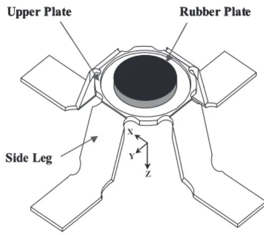
࠮ࡦࠨ⚛ሶߩᒻ⁁ࠍ

Fig. 1

ߦ␜ߔ㧚࠮ࡦࠨ⚛ሶߩ

᧚ᢱߪ㤛㌃

(C2108)

ߢ޽ࠅ㧘਄ㇱߩ᧼߇㧠ᧄ⿷ߢᡰ߃ ࠄࠇߚ᭴ㅧߣߥߞߡ޿ࠆ㧚࠮ࡦࠨ⚛ሶߩᄢ߈ߐߪ㐳 ߐ

25mm

㧘᏷

25mm

㧘㜞ߐ

10mm

ߢ޽ࠆ㧚࠮ࡦࠨ⚛

ሶߪ૞↪ߔࠆജࠍ⴫㕙ߦ⾍ࠄࠇߚᱡࠥ࡯ࠫߩ㔚᳇ᛶ

᛫ᄌൻߣߒߡᬌ಴ߔࠆ㧚਄㕙᧼ߦߪ

Z

ゲᣇะߦ૞↪

ߔࠆജࠍ⸘᷹ߔࠆߚ߼ߩᱡࠥ࡯ࠫࠍ⾍ࠅ㧘

4

ᧄߩ⿷

ߩㇱಽߦߪ

X

㧘

Y

ゲᣇะߦ૞↪ߔࠆജࠍ⸘᷹ߔࠆᱡ

ࠥ࡯ࠫࠍ⾍ࠆ㧚ߎࠇߦࠃࠅ࠮ࡦࠨ⚛ሶߪ

3

ಽജࠍ⸘

᷹ߔࠆߎߣ߇ߢ߈ࠆ㧚

X

㧘

Y

㧘

Z

ゲᣇะࠍᬌ಴ߔࠆᱡ

ࠥ࡯ࠫߦߪ㧘ฦゲߏߣߦࡉ࡝࠶ࠫ࿁〝߇⚵߹ࠇ㧘Ꮕ

േ㔚࿶ࠍ⸘᷹ߔࠆߎߣߢ૞↪ജࠍ⸘᷹ߒߡ޿ࠆ㧚㧠 ᧄ⿷ߩ਄ਅ᛬ࠅᦛߍㇱߦߪߊ߮ࠇࠍߟߌ㧘

X

ゲᣇะ

߽ߒߊߪ

Y

ゲᣇะߦജ߇૞↪ߒߚᤨߦ

Y

ゲᣇะ߽ߒ ߊߪ

X

ゲᣇะߩ㧞ᧄߩ⿷ߦ↢ߓࠆᱡࠍዊߐߊߒ㧘⋧

੕ᐓᷤࠍዊߐߊߒߡ޿ࠆ㧚߹ߚ਄㕙ߦߪ㧘ࠧࡓ᧼߇ ធ⌕ߐࠇߡ߅ࠅ㧘

Z

ゲᣇะߩ૞↪ജ߇਄㕙᧼ౝߢ╬

ಽᏓߦߥࠆࠃ߁ߦߒߡ޿ࠆ㧚

࠮ࡦࠨ⚛ሶߦജ߇૞↪ߒߚᤨ㧘࠮ࡦࠨ⚛ሶߩᄌᒻ ߪᱡࠥ࡯ࠫࠍ⾍ࠅઃߌߚ୘ᚲߩߺߢ޽ࠆߎߣ߇ᦸ߹

ߒߊ㧘߹ߚ᭴ㅧ߇ᄢ߈ߊᄌᒻߒߥ޿ᔅⷐ߇޽ࠆߚ߼㧘

࠮ࡦࠨ⚛ሶߪ೰ᕈߩ㜞޿᧚ᢱߦធ⌕ߒߡ޿ࠆ㧚

X

Y Z X

Y Z

Upper Plate Rubber Plate

Side Leg

X

Y Z X

Y Z

Side Leg

Fig. 1. Shape of sensor element

ಽᏓဳਃゲജ࠮ࡦࠨߩ᭴ㅧ

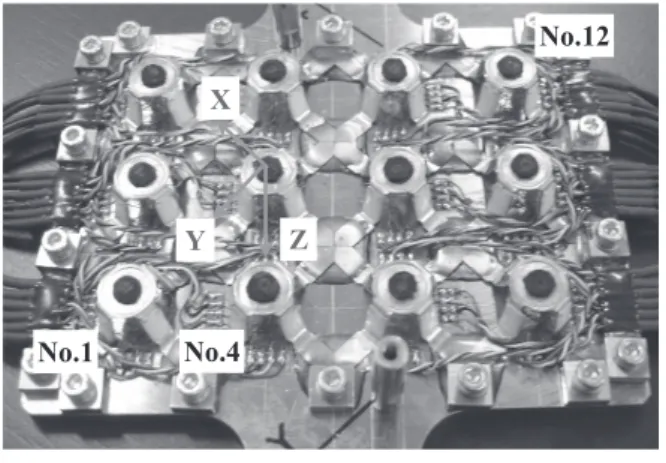
⹜૞ߒߚ࠮ࡦࠨࠍ

Fig. 2

ߦ␜ߔ㧚ߎߩಽᏓဳਃゲ ജ࠮ࡦࠨߪ㧘࠮ࡦࠨ⚛ሶࠍห৻ᐔ㕙

75mm

100mm

ߩ㕙Ⓧౝߦ

3

4

୘㈩೉ߒߚ߽ߩߢ޽ࠆ㧚࠮ࡦࠨ⚛ሶ ߩ㈩೉ߦ㑐ߒߡߪ㧘ฦ࠮ࡦࠨ⚛ሶߩ

X

㧘

Y

ゲᣇะ߇ ᐔⴕߦߥࠆࠃ߁ߦ㈩⟎ࠍⴕ޿㧘࠮ࡦࠨߣฦ࠮ࡦࠨ⚛

ሶߩ

X

㧘

Y

㧘

Z

ゲᣇะࠍ৻⥌ߐߖߡ޿ࠆ㧚ฦ࠮ࡦࠨ

⚛ሶߪု⋥ജߣߖࠎᢿജ߇⸘᷹น⢻ߢ޽ࠆߩߢ㧘ߎ ߩ࠮ࡦࠨߪ㧟ಽജߩಽᏓᖱႎࠍ⸘᷹ߔࠆߎߣ߇น⢻

ߦߥࠆ

.

ߎߎߢ㧘࠮ࡦࠨ⚛ሶߩ⇟ภࠍ

Fig. 2

ߩᏀ߆ࠄ

1

೉

⋡ߩਅ߆ࠄ

No.1

㧘

No.2

㧘

No.3

ߣߒ㧘Ꮐ߆ࠄ

2

೉⋡ߩ ਅ߆ࠄ

No.4

㧘

No.5

㧘

No.6

㧘Ꮐ߆ࠄ

3

೉⋡ߩਅ߆ࠄ

No.7

㧘

No.8

㧘

No.9

㧘Ꮐ߆ࠄ

4

೉⋡ߩਅ߆ࠄ

No.10

㧘

No.11

㧘

No.12

ߣߔࠆ㧚߹ߚ㧘ᧄ⎇ⓥߢߪ࠮ࡦࠨߩᐳ

(3)

ᮡ♽ࠍ No.5 ߩ૏⟎ࠍේὐߣߒ㧘 No.5 ߩ X 㧘 Y 㧘 Z ゲ ᣇะࠍ࠮ࡦࠨߩᐳᮡ♽ߣห৻ߣߥࠆ᭽ߦ⸳ቯߔࠆ㧚

ᧄ࠮ࡦࠨߩ࠮ࡦࠨ⚛ሶߩ઀᭽ࠍ Table 1 ߦ␜ߔ㧚♖

ᐲߪฦᣇะߩቯᩰ಴ജ୯ߦኻߔࠆ⊖ಽ₸㧔 %RO 㧕ߢ

᳞߼㧘 12 ୘ߩ࠮ࡦࠨ⚛ሶߩᐔဋ୯㧘ᮡḰ஍Ꮕ㧔 SD 㧕 ߢ␜ߒߡ޿ࠆ㧚

Fig. 2. Overview of sensor

Table 1. Specifications of sensor elements X-, Y-axis Z-axis Rated force [N] 14.7 49.0 Accuracy [%RO]

(SD)

3.79 (0.91)

0.55 (0.54)

㧚 ⸅ⷡᖱႎಣℂࠕ࡞ࠧ࡝࠭ࡓ

ฦ࠮ࡦࠨ⚛ሶߪု⋥ജ㧘ߖࠎᢿജࠍ᷹ቯߔࠆߎߣ ߇น⢻ߢ޽ࠆߩߢ㧘ᧄ࠮ࡦࠨߪ૞↪ߔࠆജࠍ 3 ಽജ ߩಽᏓᖱႎߣߒߡ⸘᷹ߢ߈ࠆ㧚ࠃߞߡ㧘ฦ࠮ࡦࠨ⚛

ሶߩ಴ജࠍ߽ߣߦ࠮ࡦࠨో૕ߦ૞↪ߔࠆ૞↪ജ㧘૞

↪ࡕ࡯ࡔࡦ࠻㧔࠮ࡦࠨᐔ㕙ߦု⋥ߥゲ๟ࠅߩࡕ࡯ࡔ ࡦ࠻㧕ࠍ᳞߼㧘Ṗࠅࠍᬌ಴ߔࠆ⸅ⷡᖱႎಣℂࠕ࡞ࠧ

࡝࠭ࡓࠍ૞ᚑߔࠆ㧚ߎߎߢ㧘ṖࠅߪࡒࠢࡠߥṖࠅߣ ࡑࠢࡠߥṖࠅߦಽߌࠄࠇࠆ㧚ࡒࠢࡠߥṖࠅߪṖࠅߩ

ೋᦼ⁁ᘒߢ⴫ࠇ㧘ࡒࠢࡠߥṖࠅ߇᜛ᄢߒࡑࠢࡠߥṖ ࠅߔߥࠊߜ࠮ࡦࠨߣធ⸅‛૕ߩ⋧ኻ⊛ߥṖࠅߣߥࠆ㧚 ࡒࠢࡠߥṖࠅߣࡑࠢࡠߥṖࠅߪㅪ⛯⊛ߦ⿠ߎࠆ⃻⽎

ߢ޽ࠅ㧘ࡒࠢࡠߥṖࠅࠍ⸘᷹ߔࠇ߫ࡑࠢࡠߥṖࠅࠍ

੍᷹ߔࠆߎߣ߇ߢ߈ࠆ㧚⃻࿷㧘ࡒࠢࡠߥṖࠅߩᬌ಴

ᣇᴺߣߒߡᨵエߥ⚛᧚ߩਛߦࡇࠛ࠱ࡈࠖ࡞ࡓࠍၒ߼

ㄟߺ㧘ࡇࠛ࠱ࡈࠖ࡞ࡓߢᓧࠄࠇࠆᝄേᖱႎߦࠃࠅࡒ

ࠢࡠߥṖࠅࠍᬌ಴ߒߡ޿ࠆ

¹¹⁾

㧚ߒ߆ߒ㧘ߎߩᣇᴺߢ ߪṖࠅᣇะࠍᬌ಴ߔࠆߎߣ߇ߢ߈ߥ޿㧚ߘߎߢᧄ⎇

ⓥߢߪฦ࠮ࡦࠨ⚛ሶߦ⾍ࠄࠇߚᱡࠥ࡯ࠫߩ಴ജ୯ߩ ᝄേᖱႎ߆ࠄࡒࠢࡠߥṖࠅࠍᬌ಴ߒ㧘Ṗࠅᣇะߪ࠮

ࡦࠨ⚛ሶߩߖࠎᢿജᣇะߩ಴ജ୯ࠃࠅᬌ಴ߔࠆߎߣ ࠍ⹜ߺࠆ㧚

ᓥߞߡ㧘⸅ⷡᖱႎಣℂࠕ࡞ࠧ࡝࠭ࡓߪធ⸅‛૕߆ ࠄฃߌࠆജ㧘ࡕ࡯ࡔࡦ࠻㧘ࡒࠢࡠߥṖࠅߣࡑࠢࡠߥ Ṗࠅߦᵈ⋡ߔࠆߣએਅߩ႐วಽߌ߇ᔅⷐߢ޽ࠆ㧚 Case (1) 3 ಽജ߇૞↪ߔࠆ႐ว

Case (2) ࡕ࡯ࡔࡦ࠻߇૞↪ߔࠆ႐ว

Case (3) Case (1) ߦട߃ਗㅴṖࠅ↢ߓࠆ႐ว Case (4) Case (2) ߦട߃࿁ォṖࠅ↢ߓࠆ႐ว

Case (5) ࡑࠢࡠߥṖࠅ㧔ਗㅴṖࠅ㧘࿁ォṖࠅ㧕߇↢

ߓࠆ⋥೨ߦࡒࠢࡠߥṖࠅ߇↢ߓࠆ႐ว ߎߩ 5 ߟ႐วߦ߅޿ߡ㧘ߘࠇߙࠇ⸅ⷡᖱႎಣℂࠕ࡞

ࠧ࡝࠭ࡓࠍ૞ᚑߔࠆ㧚

%CUGߩ⸅ⷡᖱႎಣℂࠕ࡞ࠧ࡝࠭ࡓ

Case (1) ߩ⸅ⷡᖱႎಣℂࠕ࡞ࠧ࡝࠭ࡓߢߪ㧘࠮ࡦࠨ

ߦ૞↪ߔࠆ૞↪ജࠍ Z ゲᣇะߩ૞↪ജߩ࿶ജਛᔃὐ ߦ૞↪ߒߡ޿ࠆ߽ߩߣߒߡ᳞߼ࠆ

¹²⁾

㧚

࿶ജਛᔃὐࠍ᳞߼ࠆࠕ࡞ࠧ࡝࠭ࡓࠍ␜ߔ㧚߹ߕ㧘 12 ୘ߩ࠮ࡦࠨ⚛ሶߩ಴ജࠍᑼ (3-1) ߦ␜ߔ㧚

xi yi zi

t

i f f f

f

i 112

(3-1)

ࠃߞߡ㧘࠮ࡦࠨߦ௛ߊ૞↪ജߪᑼ

_(3-2)

ߣߥࠆ㧚

¦

¹²

1 12

1 , ,

i zi

i yi z i xi y

x f F f F f

F (3-2)

ߎߎߢ㧘ේὐ๟ࠅߩജߩࡕ࡯ࡔࡦ࠻ࠍ⠨߃ࠆ㧚ේὐ ߆ࠄฦ࠮ࡦࠨ⚛ሶ߹ߢߩࡌࠢ࠻࡞ࠍ

_r_i

ߣߔࠆߣ㧘

r f

i j k

M _x _y _z

i iu i M M M

¦

¹²

1 (3-3)

ߣߥࠆ㧚ᰴߦ࿶ജਛᔃὐ

_G

ߩᐳᮡࠍ㧘

x, y, z XG,YG,0

(3-4)

ߣߒߡ㧘࿶ജਛᔃὐ๟ࠅߩജߩࡕ࡯ࡔࡦ࠻ࠍ᳞߼ࠆ㧚

࿶ജਛᔃὐ

_G

߆ࠄߩฦࠛ࡟ࡔࡦ࠻߹ߢߩࡌࠢ࠻࡞

ࠍ

_rc

ߣߒ㧘ේὐ߆ࠄ࿶ജਛᔃὐ

_G

߹ߢߩࡌࠢ࠻࡞ࠍ

R

ߣߔࠆߣ㧘࿶ജਛᔃὐ๟ࠅߩജߩࡕ࡯ࡔࡦ࠻

_M_G

ߪᑼ

_(3-5)

ߣߥࠆ㧚

No.1

No.12

No.4

Y Z

X

(4)

^

i j k

`

k j i

f R f

r f

r M

x G y G z G z G

z y x

i i

i i i

G

F Y F X F X F Y

M M M

u u

cu

¦ ¦

¦

¹²

1 12

1

(3-5)

MG

ߩ

_X

㧘

_Y

ゲᣇะᚑಽߪ࠯ࡠߣߥࠆߎߣࠃࠅ㧘࿶

ജਛᔃὐ

_G

ߩ૏⟎ߪ㧘

_¸¸

¹

·

¨¨©

§ , ,0 ,

,

z x z

y

F M F z M y

x (3-6)

ߣߥࠆ㧚

ࠃߞߡ㧘

_{Case (1)}

ߪ࿶ജਛᔃὐߦ૞↪ߔࠆജߣߒߡ

᳞߼ࠄࠇࠆ㧚

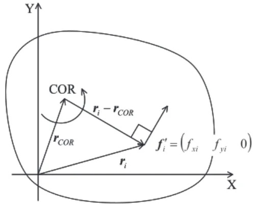
ฦ࠮ࡦࠨ⚛ሶߩ಴ജ୯ࠃࠅ࿁ォਛᔃ

_(COR)

ࠍ᳞߼㧘 ߘߩ࿁ォਛᔃߦࡕ࡯ࡔࡦ࠻߇૞↪ߒߡ޿ࠆߣߔࠆ㧚 ฦ࠮ࡦࠨ⚛ሶߩ಴ജ୯ߣ࿁ォਛᔃߩ㑐ଥࠍ

_{Fig. 3}

ߦ

␜ߔ㧚

_{Fig. 3}

ߩ㑐ଥࠃࠅᑼ

_(3-7)

߇ᓧࠄࠇࠆ㧚

f_xi f_yi

0

r_ir_COR

0 (3-7)

ᑼ (3-7) ߩ㑐ଥ߇ฦ࠮ࡦࠨ⚛ሶߦኻߒߡᚑࠅ┙ߟߎߣ

ࠃࠅ㧘࿁ォਛᔃࠍ᳞߼ࠆߎߣ߇น⢻ߣߥࠆ㧚ᓥߞߡ㧘 ߎߩ࿁ォਛᔃߦ૞↪ߒߡ޿ࠆࡕ࡯ࡔࡦ࠻ߪ㧘ᑼ (3-8) ߦࠃࠅ᳞߹ࠆ㧚

¦

¹² ^u

1

0

i xi yi i COR

t

COR f f r r

M

(3-8)

એ਄ࠃࠅ㧘 Case (2) ߪ࿁ォਛᔃߦ૞↪ߔࠆࡕ࡯ࡔࡦ࠻

ߣߒߡ᳞߼ࠄࠇࠆ㧚 Case (1) ߣ Case (2) ߩ⼂೎ߪ㧘ฦ

࠮ࡦࠨ⚛ሶߦ૞↪ߔࠆ X 㧘 Y ゲᣇะߩജߩะ߈ߦࠃ ࠅⴕ߁㧚

Case(1) ߩ⸅ⷡᖱႎಣℂࠕ࡞ࠧ࡝࠭ࡓߣห᭽ߦ࿶

ജಽᏓߩਛᔃὐࠍ᳞߼㧘ߘߩ࿶ജਛᔃὐߩ⒖േ߆ࠄ㧘 ਗㅴ⒖േ〒㔌㧘Ṗࠅᣇะࠍ᳞߼ࠆ

¹³⁾

㧚

ᤨ㑆

_t

ߢߩ࿶ജਛᔃὐ

G

ߩ૏⟎ࠍᑼ (3-9) ߣߔࠆߣ㧘 ਗㅴṖࠅߩ⒖േ〒㔌

d_G t

ߪᑼ (3-10) 㧘Ṗࠅᣇะ

D

ߪ ᑼ (3-11) ߣߥࠆ㧚

xt

,

yt

,

zt

XG

t

,

YG t

, 0 (3-9)

^

X t X t t

`

²

^

Y t Y

t t

`

²

t

d_G _G _G ' _G _G '

(3-10)

Fig. 3. Relationship between output values of sensor element and center of rotation

¸ ¸

¸

¹

· ¨ ¨

¨

©

§

¦

12 1 12 1 1

tan

i xi

i yi

f

D f (3-11)

ߎࠇߦࠃࠅ㧘ធ⸅‛૕ߩਗㅴṖࠅߩ⹏ଔ߇น⢻ߦߥ ࠅ㧘⒖േ〒㔌㧘Ṗࠅᣇะࠍ᳞߼ࠆߎߣ߇ߢ߈ࠆ㧚

࿁ォṖࠅࠍធ⸅ࡄ࠲࡯ࡦߩᘠᕈਥゲᣇะߩᄌൻߦ ࠃࠅᬌ⍮ߔࠆ㧚߹ߕ㧘ធ⸅ࡄ࠲࡯ࡦߩ࿶ജਛᔃὐߦ 㑐ߔࠆᘠᕈ࠹ࡦ࠰࡞ߪᑼ (3-12) ߣߥࠆ㧚

¸¸

¸

¹

·

¨¨

¨

©

§

Ozz Oyy Oyx

Oxy Oxx O

I I I

I I

0 0

I (3-12)

ᘠᕈਥゲ

_I_x_c

㧘

I_yc

㧘

_I_z_c

㧘ߣᘠᕈਥゲᣇะT ࠍ↪޿ߡ ᑼ

_(3-12)

ࠍ␜ߔߣ㧘ᑼ

_(3-13)

ߣߥࠆ㧚

T

T R

R

I ^t

z y x O

I I I

¸¸

¸

¹

·

¨¨

¨

©

§

c c c

0 0

(3-13)

ߚߛߒ㧘

_R_T

ߪ

_Z

ゲ๟ࠅߩࠝࠗ࡜࡯ⷺߩ࿁ォⴕ೉ߢ޽

ࠆߩߢ㧘ᑼ

_(3-14)

ߣߥࠆ㧚

¸¸

¸

¹

·

¨¨

¨

©

§

1 0 0

0 cos sin

0 sin cos

T T

RT (3-14)

ߎߎߢ㧘ᑼ

_(3-13)

㧘

_(3-14)

ࠃࠅᘠᕈਥゲᣇะT ߪએਅ ߩࠃ߁ߦߥࠆ㧚

¸¸

¹

·

¨¨

©

§

xx yy

xy

I I

2I 2tan

1 1

T _(3-15)

COR

ri

rCOR

COR

i r

r

_xi _yi 0

ic f f

f

X Y

COR

ri

rCOR

COR

i r

r

_xi _yi 0

ic f f

f

X Y

(5)

ᑼ

_(3-15)

ࠃࠅ㧘ᤨ㑆

_t

ߢߩធ⸅ࡄ࠲࡯ࡦߩ࿁ォⷺᐲߪ એਅߩࠃ߁ߦߥࠆ㧚

t t t t

d_T T T ' _(3-16)

ߎࠇߦࠃࠅ㧘࿁ォṖࠅ߇↢ߓߚ႐วߩ࿁ォㆇേߩ⹏

ଔ߇น⢻ߣߥࠆ㧚

ࡒࠢࡠߥṖࠅߪ

_{Fig. 4}

ߦ␜ߔࡈࠖ࡯࠼ࡈࠜࡢ࡯࠼

ဳ࠾ࡘ࡯࡜࡞ࡀ࠶࠻ࡢ࡯ࠢࠍ೑↪ߒߡᬌ಴ࠍⴕ߁㧚 ߎߎߢឭ᩺ߔࠆ࠾ࡘ࡯࡜࡞ࡀ࠶࠻ࡢ࡯ࠢߪࡒࠢࡠߥ Ṗ ࠅ ߇ ↢ ߓ ߡ ޿ ࠆ ߆ ߤ ߁ ߆ ߩ ߺ ࠍ ᬌ ಴ ߔ ࠆ 㧚

k

yi

i 1,2,,n

ࠍ╙

k

ጀ߆ࠄߩ಴ജ㧘 Z

_ij^k¹^,^k

^ߪ⚿ว⩄

㊀㧘

T_j

ࠍ㑣୯ߣߔࠆߣ㧘࠾ࡘ࡯࡜࡞ࡀ࠶࠻ࡢ࡯ࠢߩ ฦጀߦ߅ߌࠆ౉಴ജ㑐ଥߪ㧘ᑼ

_(3-17

㧕㧘

_(3-18)

ߣߥࠆ㧚

౉ജ㧦

ⁿ _i^k

i k k ij k

i y

x

¦

Z ¹^, (3-17)

಴ജ㧦

_y_i^k _f _x_i^k _(3-18)

ߎߎߢ㧘

f x

ߪવ㆐㑐ᢙߣ๭߫ࠇ㧘৻⥸ߦන⺞Ⴧട 㑐ᢙߢ޽ࠆ㧚ᧄ⎇ⓥߢߪਛ㑆ጀߩવ㆐㑐ᢙߣߒߡᑼ

(3-19)

ࠍ↪޿ߚ㧚

erx

x

f

1

_(3-19)

ߚߛߒ㧘

_r

ߪᱜߩછᗧଥᢙߢ޽ࠆ㧚߹ߚ಴ജጀߩવ

㆐㑐ᢙߣߒߡߪ✢ᒻ㑐ᢙࠍ↪޿ߚ㧚

ߎߩ࠾ࡘ࡯࡜࡞ࡀ࠶࠻ࡢ࡯ࠢߩ౉ജߦߪ㧘ᑼ

_(3-20)

ߦ␜ߔฦ࠮ࡦࠨ⚛ሶߩ

_Z

ᣇะߩ಴ജ୯ߩ

_FFT

ᚑಽࠍ

↪޿ࠆ㧚

Nkl N j

l zil

i k ¹f e ² ^/

0

¦

S

R k ,12,,N (3-20)

ߎߩ

_R_i _k

ߪฦ࠮ࡦࠨ⚛ሶߩ

_Z

ᣇะߩ಴ജ୯

_f_zi

ߩᤨ

㑆

_t₂₅₅'_t

߆ࠄᤨ㑆

_t

߹ߢߩ

_N ₂₅₆

୘ߩ୯ࠍ↪޿

ߡ⸘▚ߐࠇࠆ㧚ߎߩ

_R_i _k

ߩૐ๟ᵄᢙၞߩ

₄₀

୘ߩᚑ ಽࠍ౉ജߣߒߡ↪޿ࠆ㧚ߎߩ࠾ࡘ࡯࡜࡞ࡀ࠶࠻ࡢ࡯

ࠢߩ಴ജߪ㧘ᑼ

_(3-21)

ߣቯ⟵ߒߚ㧚

¯®

Slip Micro Noslip A_output

1

0

(3-21)

߹ߚ㧘ਗㅴṖࠅ߇↢ߓࠆ႐วߩࡒࠢࡠߥṖࠅߢߪ

ᑼ

_(3-11)

ࠍ↪޿ߡṖࠅᣇะࠍᬌ಴ߔࠆ㧚

x x x x x x

x x x x x

x ^A^output

i1 R

i 2 R

i 3 R

i 40

R ^x^x

x x x x

x x x x x x

x x x x x

x ^A^output

i1 R

i 2 R

i 3 R

i 40 R

Fig. 4. Model of the proposed feed-forward neural network

㧚 ⸅ⷡᖱႎಣℂࠕ࡞ࠧ࡝࠭ࡓߩᬌ⸽

⹜૞ߒߚಽᏓဳ⸅ⷡ࠮ࡦࠨ߇㧘࠮ࡦࠨߦ૞↪ߔࠆ ജ㧘ࡕ࡯ࡔࡦ࠻ࠍ⸘᷹ߢ߈㧘ធ⸅‛૕ߣ࠮ࡦࠨߣߩ

⋧ኻㆇേࠍ⹏ଔߔࠆߎߣ߇ߢ߈ࠆߎߣࠍታ㛎ߦࠃࠅ ᬌ⸽ߔࠆ㧚࠮ࡦࠨ⚛ሶߪ

₃

ಽജ߇᷹ቯน⢻ߢ޽ࠆߩ ߢฦ࠮ࡦࠨ⚛ሶߩ✚๺ߢ޽ࠆ࠮ࡦࠨߦ૞↪ߔࠆജߪ

⸘᷹น⢻ߥߎߣߪ᣿ࠄ߆ߢ޽ࠆ㧚ᓥߞߡ㧘ᧄ┨ߢߪ㧘

Case(2)-(5)

ߦᵈ⋡ߒታ㛎⚿ᨐࠍᬌ⸽ߔࠆ㧚

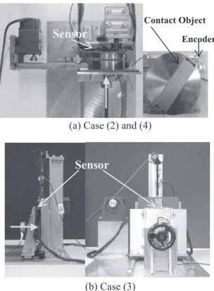
ታ㛎ᣇᴺ

Fig. 5

ߦ␜ߔⵝ⟎ࠍ↪޿ߡታ㛎ࠍⴕ߁㧚

_{Case (2)}

ߦ

߅޿ߡߪ

_{Fig. 5(a)}

ߦ␜ߔ᭽ߦ࠮ࡦࠨߦု⋥ജࠍ૞↪

ߐߖ㧘ߘߩᓟ࠮ࡦࠨߦធ⸅ߒߡ޿ࠆㇱಽࠍ࿁ォߐߖ ࠃ߁ߣߔࠆߎߣߢ࠮ࡦࠨߦࡕ࡯ࡔࡦ࠻ࠍ૞↪ߐߖࠆ㧚

Case (3)

ߦ߅޿ߡߪ

_{Fig.5 (b)}

ߦ␜ߔ᭽ߦ࠮ࡦࠨߦု⋥

ജࠍ૞↪ߐߖ㧘ߘߩᓟࡕ࡯࠲࡯ࠍ↪޿ߡ࠮ࡦࠨࠍᒁ ߈਄ߍࠆߎߣߦࠃࠅ࠮ࡦࠨߦਗㅴṖࠅࠍ↢ߓߐߖࠆ㧚

࠮ࡦࠨߩ⒖േ〒㔌ࠍᄌ૏⸘ߦࠃࠅ᷹ቯߔࠆ㧚

_{Case (4)}

ߦ߅޿ߡߪ

_{Fig. 5 (a)}

ߦ␜ߔ᭽ߦ࠮ࡦࠨߦု⋥ജࠍ૞

↪ߐߖ㧘ߘߩᓟ࠮ࡦࠨߦធ⸅ߒߡ޿ࠆㇱಽࠍ࿁ォߐ ߖࠆߎߣߢ࿁ォṖࠅࠍ↢ߓߐߖࠆ㧚ធ⸅‛૕ߩ࿁ォ

ⷺᐲߪ㧘ࠛࡦࠦ࡯࠳࡯ࠍ↪޿ߡ᷹ቯߔࠆ㧚ฦ࠮ࡦࠨ

⚛ሶߩ಴ജߪ㧘౒๺㔚ᬺ⵾ߩࠝࡦ࡜ࠗࡦဳࠦࡦ࠺ࠖ

࡚ࠪ࠽

_(MCE-24)

ࠍേᱡ᷹ቯེߣߒߡ↪޿ߡ᷹ቯߔ

ࠆ㧚

%CUGߩᬌ⸽

ೋ߼ߦ㧘

_Case(2)

ߩታ㛎⚿ᨐࠍ

_{Fig. 6}

ߦ␜ߔ㧚૞↪

ࡕ࡯ࡔࡦ࠻߇ዊߐ޿ᤨ㧘ฦ࠮ࡦࠨ⚛ሶߦ૞↪ߔࠆߖ

(6)

(a) Case (2) and (4)

(b) Case (3)

Fig. 5. Experimental equipment

ࠎᢿജᣇะߩജ߇ዊߐ޿ߚ߼᷹ቯ୯ߪ⺋Ꮕߩᓇ㗀ࠍ ᄢ߈ߊฃߌࠆ㧚ߘߩߚ߼㧘ᑼ_(3-7)ߩ㑐ଥ߆ࠄ࿁ォਛ ᔃࠍᱜ⏕ߦ᳞߼ࠄࠇߥ޿㧚ࠃߞߡ㧘_{Fig. 6} ߢߪ⸘᷹

㐿ᆎ߆ࠄ _1.7 ⑽߹ߢߩ⸘᷹୯ࠍ࠯ࡠߣߒߡ޿ࠆ㧚૞

↪ࡕ࡯ࡔࡦ࠻߇ᄢ߈ߊߥࠆߦᓥ޿චಽߥ♖ᐲߢ૞↪

ࡕ࡯ࡔࡦ࠻ࠍ⸘᷹ߢ߈ߡ޿ࠆߣ⸒߃ࠆ㧚એ਄ߩ⚿ᨐ ࠃࠅ㧘⹜૞ߒߚಽᏓဳ⸅ⷡ࠮ࡦࠨߪ㧘૞ᚑߒߚ⸅ⷡ

ᖱႎಣℂࠕ࡞ࠧ࡝࠭ࡓߦࠃࠅ૞↪ജ㧘૞↪ࡕ࡯ࡔࡦ

࠻ࠍ⸘᷹ߔࠆߎߣ߇ߢ߈ࠆߎߣ߇␜ߖߚ㧚

ᰴߦ㧘_Case(3)ߩታ㛎⚿ᨐࠍ␜ߔ㧚ߎߩታ㛎⚿ᨐߪ㧘

࠮ࡦࠨߩ_Zゲᣇะߦ⚂_14Nߩജࠍ૞↪ߐߖߚ⁁ᘒߢ X ゲᣇะ߆ࠄ ₄₅ ᐲᣇะߦਗㅴṖࠅࠍ↢ߓߐߖߚ⚿

ᨐߢ޽ࠆ㧚࿶ജਛᔃὐ_(COP)ߩ⒖േࠍ_{Fig. 7}ߦ␜ߒ㧘

⒖േ〒㔌ࠍ_{Fig. 8}ߦ␜ߔ㧚ߘߒߡ㧘⒖േᣇะࠍ_{Fig. 9}

ߦ␜ߔ㧚_{Fig. 9} ߢߪ㧘ਗㅴṖࠅ߇↢ߓࠆ߹ߢߩ⒖േ

ᣇะߩ୯ߪ࠯ࡠߣߒߡ޿ࠆ㧚ߎߩ⚿ᨐࠃࠅ㧘࿶ജਛ ᔃὐߩ⒖േ㧘⒖േ〒㔌ߣ߽ߦታ㓙ߩ࿶ജਛᔃὐߩ⒖

േ㧘⒖േ〒㔌ߣߩ⺋Ꮕ߇ᄢ߈ߊߥߞߡ޿ࠆ㗔ၞ߇ሽ

࿷ߔࠆ㧚೨┨ߢ␜ߒߚ⸅ⷡᖱႎಣℂࠕ࡞ࠧ࡝࠭ࡓߢ ߩ࠮ࡦࠨ⚛ሶߩ૏⟎ߪ࠮ࡦࠨ⚛ሶߦ⾍ࠅઃߌߡ޿ࠆ

਄ㇱߩࠧࡓߩਛᔃ૏⟎ߢቯ⟵ߒ㧘ߘߩࠧࡓߩਛᔃ૏

⟎ߦ૞↪ജ߇૞↪ߒߡ޿ࠆ߽ߩߣߒߡ޿ࠆ㧚ߒ߆ߒ㧘 ធ⸅‛૕ߦធߒߡ޿ߥ߆ߞߚ࠮ࡦࠨ⚛ሶ߇ធ⸅‛૕

߇ធߒᆎ߼ࠆ㓙㧘࠮ࡦࠨ⚛ሶߪ਄㕙ߩࠧࡓߩ┵߆ࠄ ធ⸅‛૕ߦធߒᆎ߼㧘૞↪ജࠍฃߌᆎ߼ࠆ㧚ࠃߞߡ㧘

࠮ࡦࠨ⚛ሶߦ⾍ࠅઃߌߚࠧࡓ᧼ߪ⋥ᓘ _5.0mm ߢ޽

ࠆߩߢ㧘⸅ⷡᖱႎಣℂࠕ࡞ࠧ࡝࠭ࡓߢቯ⟵ߒߚജߩ

૞ ↪ ὐߣ ฦ࠮ ࡦ ࠨ⚛ ሶߩ ታ 㓙ߩ ૞↪ ὐ ߇ᦨ ᄢߢ

2.5mmߕࠇࠆߎߣߦࠃࠅ㧘⺋Ꮕ߇↢ߓߚේ࿃ߣߥࠆ

ߣ⠨߃ࠄࠇࠆ㧚߹ߚ㧘ฦ࠮ࡦࠨ⚛ሶߩ㜞ߐߦ߫ࠄߟ ߈߇ሽ࿷ߔࠆߚ߼㧘㜞ߐߩ㜞޿࠮ࡦࠨ⚛ሶߩ૞↪ജ ߇ᄢ߈ߊߥࠅ㧘ૐ޿࠮ࡦࠨ⚛ሶߢߪዊߐߊߥߞߚߚ

߼ታ㓙ߩ୯ߣߩ⺋Ꮕ߇ᄢ߈ߊߥߞߚߣ⠨߃ࠄࠇࠆ㧚 ߒ߆ߒ㧘ฦ࠮ࡦࠨ⚛ሶߩ㑆ߩᦨ⍴〒㔌߇_25.0㨙㨙ߦ

߽߆߆ࠊࠄߕߘࠇએਅߩធ⸅‛૕ߩਗㅴㆇേࠍᝒ߃ ࠆߎߣ߇ߢ߈ߡ޿ࠆߣ⸒߃㧘ਗㅴṖࠅߩᬌ⍮߇น⢻

ߢ޽ࠆߎߣࠍ␜ߒߡ޿ࠆ

Fig. 6. Measured result of applied moment

Fig. 7. Measured result of COP

-0.5 0 0.5 1 1.5 2 2.5 3

X [mm]

Y [mm]

Calculated COP Actual COP

-0.5 0 0.5 1 1.5 2 2.5 3

X [mm]

Y [mm]

Calculated COP Actual COP Calculated COP Actual COP Calculated COP Actual COP

0 1 2 3 4 5 6 7

-5 0 5 10 15 20

Time [s]

Moment [Nmm]

Calculated Moment Applied Moment

0 1 2 3 4 5 6 7

-5 0 5 10 15 20

Time [s]

Moment [Nmm]

Calculated Moment Applied Moment Calculated Moment Applied Moment Calculated Moment Applied Moment

Sensor

Contact Object Encoder

Sensor

(7)

Fig. 8. Measured result of displacement of COP

Fig. 9. Measured result of slip direction

ᦨᓟߦ㧘_Case(4)ߩታ㛎⚿ᨐߢ޽ࠆ࿁ォⷺᐲߩ⸘᷹

⚿ᨐࠍ_{Fig. 10}ߦ␜ߔ㧚ߎߩታ㛎⚿ᨐߪ㧘࠮ࡦࠨߩ_Z

ゲᣇะߦ⚂_81Nߩജࠍ૞↪ߐߖߚ⁁ᘒߢ࿁ォṖࠅࠍ

↢ߓߐߖߚ⚿ᨐߢ޽ࠆ㧚ߎߩ⚿ᨐߦ߅޿ߡ㧘ታ㓙ߩ

࿁ォⷺᐲߣ⸅ⷡᖱႎಣℂࠕ࡞ࠧ࡝࠭ࡓߦࠃࠅ᳞߼ߚ

࿁ォⷺᐲߢߪᦨᄢ_0.84ᐲߩ⺋Ꮕ߇↢ߓߡ޿ࠆ㧚ߎߩ

⺋Ꮕ߽ਗㅴṖࠅߢ↢ߓߚ⺋Ꮕߣห᭽ߦ㧘ቯ⟵ߒߚജ ߩ૞↪ὐߣฦ࠮ࡦࠨ⚛ሶߢߩታ㓙ߩജߩ૞↪ὐߩߕ ࠇߦࠃࠆᓇ㗀ߣฦ࠮ࡦࠨ⚛ሶߩ㜞ߐߩ߫ࠄߟ߈ߦࠃ ࠆᓇ㗀ߢ޽ࠆߣ⠨߃ࠄࠇࠆ㧚ߒ߆ߒ㧘ធ⸅‛૕ߦ࿁

ォṖࠅ߇↢ߓߚ႐วߩ࿁ォⷺᐲࠍචಽߥ♖ᐲߢ᳞߼

ࠆߎߣߢ߈ࠆߣ⸒߃㧘࿁ォṖࠅ߇ᬌ⍮น⢻ߢ޽ࠆߎ ߣࠍ␜ߒߡ޿ࠆ㧚

એ਄ߩ⚿ᨐࠃࠅ㧘ᧄ࠮ࡦࠨߪ㧘૞↪ജ㧘૞↪ࡕ࡯

ࡔࡦ࠻ߩ⸘᷹ߔࠆߎߣ߇น⢻ߢ޽ࠅ㧘ࡑࠢࡠߥṖࠅ ߩᬌ಴߇น⢻ߢ޽ࠆߎߣ߇␜ߐࠇߚ㧚

Fig. 10. Measured result of rotation angle

%CUGߩᬌ⸽

ࡒࠢࡠߥṖࠅ߇↢ߓߡ޿ࠆ▎ᚲߦᵈ⋡ߔࠆߣ㧘ࡒ

ࠢࡠߥṖࠅߪਗㅴṖࠅߣ࿁ォṖࠅߣߩᏅ⇣ߪߥ޿㧚 ᓥߞߡ㧘ᧄ⺰ᢥߢߪਗㅴṖࠅᤨߩࡒࠢࡠߥṖࠅߩᬌ

಴ࠍ଀ߦ᜼ߍ㧘⸅ⷡᖱႎಣℂࠕ࡞ࠧ࡝࠭ࡓߩ᦭ലᕈ ߩᬌ⸽ࠍⴕߞߚ㧚

ቇ⠌ㆊ⒟

ࡒࠢࡠߥṖࠅᬌ಴ࠍⴕ߁೨ߦ૞ᚑߒߚ࠾ࡘ࡯࡜࡞

ࡀ࠶࠻ࡢ࡯ࠢߩቇ⠌ࠍⴕ߁㧚ᢎᏧାภߩ૞ᚑߦߪ㧘 ᄌ૏࠮ࡦࠨߩ಴ജࠍၮߦ૞ᚑߒߚ㧚ਗㅴṖࠅࠍ↢ߓ ߐߖࠆ੍஻ታ㛎ࠍⴕ޿㧘੍஻ታ㛎ߩ⚿ᨐ߆ࠄᢎᏧା

ภᢎᏧାภࠍ૞ᚑߒߚ㧚_{Fig. 11}ߪ੍஻ታ㛎ߩਗㅴ⒖

േ〒㔌ߩ⸘᷹⚿ᨐߢ޽ࠅ㧘_{Fig. 12} ߪ੍஻ታ㛎ᤨߩ No.8ߩ࠮ࡦࠨ⚛ሶߩ_Zゲᣇะߩ಴ജ୯ߩࠬࡍࠢ࠻࡞

ࠣ࡜ࡓߢ޽ࠆ㧚_{Fig. 11}ߩ⚿ᨐ߆ࠄ⚂_2.5⑽ߦࡑࠢࡠ ߥṖࠅ߇↢ߓߡ޿ࠆߎߣ߇ࠊ߆ࠆ㧚ߘߒߡ㧘_{Fig. 12} ߩ⚿ᨐ߆ࠄ㧘_2.2⑽߆ࠄ_2.5⑽߹ߢߩ㑆ߦᝄേ߇↢ߓ ߡ޿ࠆߎߣ߇ࠊ߆ࠆ㧚ߎߩ㑆ߦࡒࠢࡠṖࠅ߇߅߈ߡ

޿ࠆߎߣ߇ࠊ߆ࠆ㧚ߎߩ⚿ᨐࠃࠅᢎᏧାภߩ಴ജࠍ

૞ᚑߒቇ⠌ࠍⴕߞߚ㧚࠾ࡘ࡯࡜࡞ࡀ࠶࠻ࡢ࡯ࠢߩቇ

⠌ߦߪ㧘ㅙᰴᦝᣂቇ⠌ᴺߩ㧝ߟߢ޽ࠆࡃ࠶ࠢࡊࡠࡄ

ࠥ࡯࡚ࠪࡦᴺࠍ↪޿ߚ㧚

ࡒࠢࡠߥṖࠅߩᬌ಴⚿ᨐ

ࡒࠢࡠߥṖࠅࠍ૞ᚑߒߚ࠾ࡘ࡯࡜࡞ࡀ࠶࠻ࡢ࡯ࠢ

ߦࠃࠅᬌ⍮น⢻߆ࠍታ㛎ߦࠃࠅᬌ⸽ߔࠆ㧚

Ṗࠅᬌ⍮ߩ಴ജߪᑼ_(4-1)ߩ᭽ߦቯ⟵ߒ㧘_{Fig. 13}ߦ

0 2 4 6 8 10 12

Time [s]

T [degree]

Calculated Rotation Angle Actual Rotation Angle

0 2 4 6 8 10 12

Time [s]

T [degree]

Calculated Rotation Angle Actual Rotation Angle Calculated Rotation Angle Actual Rotation Angle Calculated Rotation Angle Actual Rotation Angle

0 1 2 3 4 5 6 7

0 10 20 30 40 50

Time [s]

D [degree]

Calculated Slip Direction Actual Slip Direction

0 1 2 3 4 5 6 7

0 10 20 30 40 50

Time [s]

D [degree]

Calculated Slip Direction Actual Slip Direction Calculated Slip Direction Actual Slip Direction Calculated Slip Direction Actual Slip Direction

0 1 2 3 4 5 6 7

0 1 2 3 4

Time [s]

Displacement [mm]

Calculated Displacement Actual Displacement

0 1 2 3 4 5 6 7

0 1 2 3 4

Time [s]

Displacement [mm]

Calculated Displacement Actual Displacement Calculated Displacement Actual Displacement Calculated Displacement Actual Displacement

(8)

Fig. 11. Measured result of displacement

Fig. 12. Spectrogram of the No. 8 sensor element’s output in Z-axis direction

␜ߔᚻ㗅ߢṖࠅᬌ⍮ࠍⴕߞߚ㧚

°¯

°®

Slip al Tranlation of

Slip Macro

Slip Micro Noslip Soutput

2 1 0

(4-1) ታ㛎⚿ᨐࠍFig. 14- Fig. 16ߦ␜ߔ㧚_{Fig. 14}ߪᄌ૏

⸘ߩ಴ജ෸߮ _COP ߩਗㅴ⒖േ〒㔌ߢ޽ࠆ㧚_{Fig. 15} ߪṖࠅᬌ⍮⚿ᨐߢ޽ࠆ㧚ߘߒߡ㧘_{Fig. 16}ߪਗㅴ⒖േ

ᣇะࠍ␜ߒߡ޿ࠆ㧚ਗㅴ⒖േᣇะߪࡒࠢࡠߥṖࠅ߇ ᬌ಴ߐࠇࠆ߹ߢߪ࠯ࡠߣߒߡ޿ࠆ㧚ߎࠇߦࠃࠅ㧘૞

ᚑߒߚ࠾ࡘ࡯࡜࡞ࡀ࠶࠻ࡢ࡯ࠢߪࡒࠢࡠߥṖࠅࠍᬌ

⍮ߔࠆߎߣ߇ߢ߈ߡ޿ࠆ㧚߹ߚ㧘_{Fig. 16}ߦᵈ⋡ߔࠆ ߣᓥ᧪ߩ⸅ⷡ࠮ࡦࠨߢߪᬌ಴ߢ߈ߥ߆ߞߚࡒࠢࡠߥ Ṗࠅ߇↢ߓߚᤨߩṖࠅᣇะ߽ᬌ಴ߢ߈ߡ޿ࠆߎߣ߇

ࠊ߆ࠆ㧚

એ਄ࠃࠅ㧘ᧄ࠮ࡦࠨࠪࠬ࠹ࡓߪࡒࠢࡠߥṖࠅߣࡑ

ࠢࡠߥṖࠅࠍㅪ⛯ߒߡᓧࠆ੐߇น⢻ߢ޽ࠆߎߣ߇␜

ߐࠇߚ㧚

Fig. 13. Flow chart of slip detection

Fig. 14. Measured result of COP displacement

Fig. 15. Result of slip detection Time [s]

Frequency [Hz]

0 1 2 3 4 5

0 50 100 150 200

䎐䎔䎓䎓䎐䎛䎓䎐䎙䎓䎐䎗䎓䎐䎕䎓䎓䎕䎓䎗䎓

Micro-slip Macro-slip

Time [s]

Frequency [Hz]

0 1 2 3 4 5

0 50 100 150 200

䎐䎔䎓䎓䎐䎛䎓䎐䎙䎓䎐䎗䎓䎐䎕䎓䎓䎕䎓䎗䎓

0 1 2 3 4 5

0 0.5 1 1.5 2

Time [s]

Displacement [mm]

0 1 2 3 4 5

0 0.5 1 1.5 2

Time [s]

Displacement [mm]

0 2 4 6 8

0 1 2 3 4

Time [s]

Displacement [mm]

Calculated Displacement Actual Displacement

0 2 4 6 8

0 1 2 3 4

Time [s]

Displacement [mm]

Calculated Displacement Actual Displacement Calculated Displacement Actual Displacement Calculated Displacement Actual Displacement Slip Detection

Output Macro-slip is

generated

output 2 S

Yes

No

i A

Soutput output

Sensor element for detecting the micro-slip

is selected Slip Detection

Output Macro-slip is

generated

output 2

Soutput 2

S

Yes

No

i A Soutput Aoutput i

Soutput output

Sensor element for detecting the micro-slip

is selected Sensor element for detecting the micro-slip

is selected

0 2 4 6 8

0 0.5 1 1.5 2 2.5 3

Time [s]

Slip Detection

(9)

Fig. 16. Measured result of slip direction

㧚 ⚿⸒

ᧄ⎇ⓥߢᓧࠄࠇߚ⚿⺰ߪએਅߩㅢࠅߢ޽ࠆ㧚 1㧚 ᧄ⎇ⓥߢ⹜૞ߒߚಽᏓဳ⸅ⷡ࠮ࡦࠨߪ㧘૞ᚑߒ

ߚ⸅ⷡᖱႎಣℂࠕ࡞ࠧ࡝࠭ࡓߦࠃࠅ૞↪ߔࠆ ₃ ಽജߩಽᏓᖱႎ߇⸘᷹ߢ߈㧘૞↪ߔࠆജ㧘ࡕ࡯

ࡔࡦ࠻ࠍ⸘᷹ߔࠆߎߣ߇ߢ߈ࠆ㧚

2㧚 ᧄ⎇ⓥߢ⹜૞ߒߚಽᏓဳ⸅ⷡ࠮ࡦࠨߪ㧘૞ᚑߒ ߚ⸅ⷡᖱႎಣℂࠕ࡞ࠧ࡝࠭ࡓߦࠃࠅਗㅴṖࠅࠍ

↢ߓߚធ⸅‛૕ߩ⒖േ〒㔌㧘⒖േᣇะࠍ⸘᷹ߔ ࠆߎߣ߇น⢻ߢ޽ࠆߚ߼㧘ਗㅴㆇേࠍ⹏ଔߢ߈ ࠆ㧚

3㧚 ᧄ⎇ⓥߢ⹜૞ߒߚಽᏓဳ⸅ⷡ࠮ࡦࠨߪ㧘૞ᚑߒ ߚ⸅ⷡᖱႎಣℂࠕ࡞ࠧ࡝࠭ࡓߦࠃࠅ࿁ォṖࠅࠍ

↢ߓߚធ⸅‛૕ߩ࿁ォⷺᐲࠍ⸘᷹ߔࠆߎߣ߇น

⢻ߢ޽ࠆߚ߼㧘࿁ォㆇേࠍ⹏ଔߢ߈ࠆ㧚 4㧚 ᧄ⎇ⓥߢ⹜૞ߒߚಽᏓဳ⸅ⷡ࠮ࡦࠨߪ㧘૞ᚑߒ

ߚ⸅ⷡᖱႎಣℂࠕ࡞ࠧ࡝࠭ࡓߦࠃࠅࡒࠢࡠߥṖ ࠅࠍᬌ಴ߢ߈㧘ࡑࠢࡠߥṖࠅ߇↢ߓࠆ੍᷹ߔࠆ ߎߣ߇ߢ߈ࠆ㧚

ߥ߅ᧄ⎇ⓥߩ৻ㇱߪ㧘ᣣᧄቇⴚᝄ⥝ળ⑼ቇ⎇ⓥ⾌

⵬ഥ㊄₍․೎⎇ⓥຬᅑബ⾌㧘⺖㗴⇟ภ _19-5611)෸߮

(⽷₎ ↥ቇ౏⎇ⓥ㐿⊒ᡰេ੐ᬺߩេഥࠍฃߌߚ㧚⸥ߒ ߡ⻢ᗧࠍ⴫ߔ㧚

ෳ⠨ᢥ₂

1) ૒ޘᧁᄢテ㧘ೣᰴବ㇢㧘㜞ጤ᣽ᒄ㧘_“↢ᵴᡰេࡠࡏ࠶

࠻ߩߚ߼ߩ࿶ജᬌ಴ဳ࠰ࡈ࠻⸅ⷡ࠮ࡦࠨߩ㐿⊒’’㧘ᣣ ᧄᯏ᪾ቇળ⺰ᢥ㓸 C✬㧘70-689㧘77-82 (2004).

2) ᄢጟ᣽ඳ㧘_“࿶ജಽᏓߣߖࠎᢿജߩหᤨ⸘᷹ࠍน⢻ߣ ߔࠆਃゲ⸅ⷡ࠮ࡦࠨ’’㧘ᣣᧄᯏ᪾ቇળ⹹㧘104-901㧘 372-373 (2001).

3) Antonio Bicci and Vijay Kumar, “Robotic grasping and contact: A review”, In Proceedings of the 2000 IEEE International Conference on Robotics and Automation, 348–353, (2001).

4) ೨Ꮉੳ㧘̌⸅ⷡᖱႎࠍ೑↪ߒߚᄙᜰࡂࡦ࠼ߦࠃࠆᛠ

ី࡮ᠲࠅ̍㧘ᣣᧄࡠࡏ࠶࠻ቇળ⹹㧘18-6㧘776-781 (2000).

5) ะ੗೑ᤐ㧘⟜ᔒஉ㧘ട⮮㓁㧘ઁ61ฬ㧘⿥੖ᗵ࠮ࡦࠨ ߩ㐿⊒ᦨ೨✢㧘(ᑼળ␠ ࠛ࠿࡮࠹ࠖ࡯࡮ࠛࠬ㧘᧲੩㧘 2005)㧘pp.299-309.

6) E.G.M. Holweg and W. Jongkind㧘“Object Recognition Using a Tactile Matrix Sensor’’㧘Proceedings of European Robotics and Intelligent System Comference㧘1379-1383㧘 (1994).

7) ᳗੗ᷡ㧘દ⮮⟵ౖ㧘⍫ፒ⺈㧘ᮘญసᏆ㧘㒙ㇱᥙ㧘ੑ㊀ චሼ᭴ㅧߦၮߠߊዊဳ6ಽജജⷡ࠮ࡦࠨߩ㐿⊒㧘ᣣᧄ ࡠࡏ࠶࠻ቇળ⹹㧘22-3㧘361-369 (2004).

8) H. Shinoda㧘M. Uehara and S. Ando㧘A Tactile Sensor using Three-Dimensional Structure㧘Proceedings of the 1992 IEEE International Conference on Robotics and Automation㧘217-220 (1992).

9) ෹࿡િ଻㧘⮮ၴാ㓶㧘⮳↰ື㇢㧘̌㔚⏛⺃ዉߦၮߠߊ

ਃゲ⸅ⷡ࠮ࡦࠨߣߘߩ․ᕈ̍㧘ᣣᧄᯏ᪾ቇળ⺰ᢥ㓸 C

✬㧘71-703㧘920-927 (2005).

10) ␹ጊ๺ੱ㧘Ḵ↰ᤩ৻㧘᫃ᧄ⵨ਯ㧘Ꮉ਄⋥᮸㧘⥪┨㧘̌శ ቇᑼਃᰴర⸅ⷡ࠮ࡦࠨߩࡠࡏ࠶࠻ࡈࠖࡦࠟ߳ߩㆡ↪̍㧘 ࡠࡏ࠹ࠖࠢࠬ࡮ࡔࠞ࠻ࡠ࠾ࠢࠬ⻠Ṷળ⻠Ṷ⺰ᢥ㓸㧘 2005㧘1P1-N-104 (2005).

11) ᄙ↰ᵏᓼ㧘⑔↰ᢕผ㧘⚦↰⠹㧘̌ⷞ⸅ⷡࠍᜬߟࡠࡏ࠶

࠻ࡂࡦ࠼ߦࠃࠆṖࠅ⴫⃻ߩ₪ᓧߣᜬߜ਄ߍേ૞ߩታ

⃻̍㧘ࡠࡏ࠹ࠖࠢࠬ㨯ࡔࠞ࠻ࡠ࠾ࠢࠬ⻠Ṷળ⻠Ṷ⺰ᢥ㓸㧘 2006㧘2P2-B20 (2006).

12) ጊ⿧ᙗ৻㧘ᚭᎹ㆐↵㧘㨬↢૕↪࠮ࡦࠨߣ⸘᷹ⵝ⟎㨭㧘㧔ࠦ

ࡠ࠽␠㧘᧲੩㧘2000㧕㧘110-139.

13) C. Melchiorri㧘Tactile Sensing for Robotic Manipulation㧘 Lecture Notes in Control and Information Sciences㧘270㧘 75-102 (2001).

0 2 4 6 8

0 10 20 30 40 50