著者 BIAO Wang
出版者 法政大学大学院情報科学研究科
雑誌名 法政大学大学院紀要. 情報科学研究科編
巻 12
ページ 1‑6
発行年 2017‑03‑31
URL http://doi.org/10.15002/00014019
Smoke Simulation using WebGL Technology
WANG BIAO
Graduate School of Computer and Information Sciences Hosei University
Abstract—Building smoke simulation is an important and chal- lenging task which has widely application in computer graphics.
Although use of native application can effectively visualize fluid mechanics, necessary softwares or plugins need to be installed.
Especially, if your applications releasing to many platforms such as Windows, Linux and Mac OS, you have to develop different versions for every platform. To solve these problems, this paper proposes a method to implement smoke simulation through a modern web browser using HTML5 and WebGL exclusively.
With the development of the Internet, Web-based applications have become increasingly popular in many areas and advances in web-based 3D graphics were made accordingly. In this paper, we present a web based implementation of smoke simulation, the smoke effects can be obtained in a website, of course the cross-platform problems in web-based systems can be solved.
Keywords—smoke simulation, WebGL, physical models, GPGPU
I. INTRODUCTION
A. Concepts of Navier-Stokes Equations
The smoke animators are interested in is governed by the famous incompressible Navier-Stokes equations, a set of partial different equations that are supposed to hold throughout the smoke. They are usually written as:
The traditional fingerprint authentication system adopts the following technical architecture:
∂~u
∂t +~u· ∇~u+1
ρ∇p=ν∇ · ∇~u+F (1)
∇ ·~u= 0 (2)
1) Symbols: The letter ~u is traditionally used in fluid mechanics for the velocity of the fluid. Why not~v? It is hard to say, but it fits another useful convention, to call the three components of 3D velocity (u,v,w).
The Greek letter ρ stands for the density of the fluid. For water, this is roughly 1000kg/m3 and for air this is roughly 1.3kg/m3, a ratio of about 700:1.
The letterpstands for “pressure”, the force per unit area that the fluid exerts on anything.
The Greek letter ν is technically called the “kinematic viscosity”. It measures how viscous the fluid is. Fluids like molasses have high viscosity, and fluids like alcohol have low viscosity: it measures how much the fluid resists deforming while it flows (or more intuitively, how difficult it is to stir).
The letter F is external forces applied to the fluid. More generally people call these “body forces”, because they are applied throughout the whole body of fluid, not just on the surfaces [1].
2) Terms in the Navier-Stokes Equations:
1) Advection: The velocity of a fluid causes the fluid to transport objects, densities, and other quantities along with the flow. Imagine squirting dye into a moving fluid.
The dye is transported, or advected, along the fluids velocity field. In fact, the velocity of a fluid carries itself along just as it carries the dye. The second term on the left-hand side of Equation (1) represents this self- advection of the velocity field and is called the advection term.
2) Pressure: Because the molecules of a fluid can move around each other, they tend to “squish” and “slosh”.
When force is applied to a fluid, it does not in- stantly propagate through the entire volume. Instead, the molecules close to the force push on those farther away, and pressure builds up. Because pressure is force per unit area, any pressure in the fluid naturally leads to acceleration. (Think of Newton’s second law,F =ma.) The third term on the left-hand side, called the pressure term, represents this acceleration.
3) Diffusion: From experience with real fluids, you know that some fluids are “thicker” than others. For example, molasses and maple syrup flow slowly, but rubbing alcohol flows quickly. We say that thick fluids have a high viscosity. Viscosity is a measure of how resistive a fluid is to flow. This resistance results in diffusion of the momentum (and therefore velocity), so we call the first term on the right-hand side as the diffusion term.
4) External Forces: The fourth term encapsulates acceler- ation due to external forces applied to the fluid. These forces may be either local forces or body forces. Local forces are applied to a specific region of the fluid—for example, the force of a fan blowing air. Body forces, such as the force of gravity, apply evenly to the entire fluid.
B. Motivation
The demand for exciting and elaborate, and often pro- fessional, web applications has risen to new level. To keep up with it, in recent years a lot of effort was put forth to increase the 3D graphics capabilities of web applications.
Presented solutions usually require the installation of browser add-ons in order to view the 3D content, forcing the user to install a plug-in first. To avoid such complications and make advanced 3D and 2D graphics accessible to a wide audience, in 2009 the Khronos Group started an initiative to develop a
standardized, native, low-level API based on the OpenGL ES 2.0 [2] specification, nowadays known as WebGL. WebGL allows for the rendering of 3D objects in the browser devoid of any additional software making it accessible to all internet users with WebGL enabled browsers [3].
Because the WebGL have convenience and cross-platform features. So my research is about using the WebGL technology to implement fluid simulation. After analyzing the physical equation of fluid flow named as the Navier-Stokes, we can visualize fluid mechanics by numerical simulation, at last we will look the result in real time.
II. RELATED WORK
This chapter talks about the related technology in the fluid simulation. At first, we will introduce how to use Volume Ray Casting to render 3D volume, after that, have a overview about WebGL.
A. Volume Ray Casting
1) Volume Rendering: The term volume rendering is used to describe techniques which allow the visualization of three- dimensional data. Volume rendering is a technique for vi- sualizing sampled functions of three spatial dimensions by computing 2-D projections of a colored semitransparent vol- ume. Unlike traditional rendering uses triangles to display 3D graphics, volume rendering [4] uses other methods such as Volume Ray Casting. This image-based method renders a 3D scalar field into a 2D image by casting rays along the 3D volume. Each pixel we see on the screen is the result of a ray that is going through the cube and getting intensity samples from the voxels at regular intervals.
But how do we cast rays?
A simple option is to use 3D mesh cube of size (1,1,1) and render the front and back faces (enabling and disabling back face culling) in two different render passes.
For every cube fragment generated in the screen we can create a ray that starts at the front face of cube and ends in back face. Having the starting and ending points of the ray we can start sampling the voxels at regular intervals to generate the resulting fragment color [5].
Fig. 1. The scalar field is represented as voxels that contain the intensity values at each (x,y,z) position
B. WebGL: History and Technologies
Up until recently, content on the internet has usually been a generally 2D experience. It was invented about twenty years ago to connect different nodes using hypertext (which would be standardised as HTML later on) to share reports and information from databases. 3D experiences have been achieved in online games and applications since but this is usually through the utilisation of 3D collaboration programmes that can be used as plugins in browsers. As such, the use of 3D in web browsers is usually confined to specific, non- mainstream uses.
WebGL is a lightweight software library that uses Javascript to implement OpenGL ES 2.0 commands. OpenGL ES is a subset of OpenGL that has been designed for embedded devices such as smart phones and PDAs. This allows for the 3D information drawn in the canvas element to be compatible not only with browsers on desktops but on small mobile devices too. OpenGL and OpenGL ES are published by the Khronos Group which is consortium consisting of companies that deal with graphical hardware and software such as Nvidia, Sony and Intel.
Even though WebGL is a massive improvement on what has been available through the browsers before it does have some disadvantages including resource loading limits, security limitations and event handling limitations, more information on these topics are presented by Borsos [6]. Another disad- vantage is that since WebGL is based upon OpenGL ES it does not include 3D textures (3D textures are only available in OpenGL ES through an extension). This means that the 3D texture volume rendering technique need to use 2D texture to emulate.
III. DESIGN
The aim of this project is to produce a smoke simulation application that is usable through a WebGL enabled browser at real time rates without any additional third party software.
A. Requirements
The WebGL becoming more and more popular with the development of technology that is most commonly used in game development. At now, the very famous game engine Unity also support using WebGL to develop games. Because it is very convenient and cross-platform, you just need input the website address and wait a moment, the game will be shown in your eyes. You do not need install any additional software.
Fluid flows are everywhere: from rising smoke, clouds and mist to the flow of rivers and oceans. Because one of the major goals of games is to immerse players into plausible virtual worlds, it is desirable to include fluid flows into game engines. There already exist many adhoc models that attempt to fake fluid-like effects, such as particles rendered as textured sprites. However, animating them in a convincing manner is not easy.
So I selected the smoke simulation as my research topic.
I believe that a better alternative is to use the physics of fluid flows which is the Navier-Stokes Equations, a precise mathematical model for most fluid flows occurring in Nature.
We use the numerical algorithms to solve the equations. I have to say, if you want the result with more accuracy, of course you will spend more time on the calculation. On the other hand what matters most is a realistic and fast simulation in computer graphics. So we need balance the realistic result and render speed.
B. Data Loading Technique
Finding a quick and reliable way of loading in the data for volume rendering is a very important aspect of any volume rendering application. The focus of data loading in my project is calculate and save the volume data in texture.
1) The Problem: One of the essential parts of any volume renderer is, naturally, the volume data itself. Currently, 3D textures are the most popular and convenient way to handle the volume data. This is based on the earlier explained view of a volume as a uniform, three dimensional grid. Unfortunately, there currently is no native support for 3D textures available in the WebGL Specification.
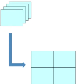
2) The Solution: A known solution for this issue is to emulate the 3D texture using the available 2D texture support [7]. This approach suggests itself, since one way to interpret a 3D texture is as a number of 2D textures. These single 2D textures, which together add up to the complete 3D texture or volume, are henceforth referred to as slices. The aim of this method is to find an optimal way to copy and arrange all slices of a given volume into a single 2D texture, often referred to as a texture atlas. Furthermore each slice should not be split into smaller parts, but remain as whole within the 2D texture space. Figure 2 illustrates the general idea of how the slices are arranged in a 2D texture.
Fig. 2. Illustrates how the slices of a volume are arranged inside a single 2D texture.
C. Our Approach
A naive algorithm could simply copy the data of the 3D texture into a 2D texture with the same width as a single
slice and the height of a slice multiplied by the number of slices as its height. Obviously this would not produce an optimal result, especially when considering the limited maximum texture resolution of graphic card hardware. Instead, a more optimal texture resolution can be found by trying to meet two conditions.
First, the widthmmultiplied by the heightnof the texture has to be either equal or greater than the volumes width x multiplied with its height y and depth z, so that there is a texel in the texture for every voxel of the volume.
Second, the width and height of the texture should be approximately the same, so that a maximum amount of image data can be fitted into a single texture file.
So, we selected use 512∗512 2D texture to emulate the 64∗64∗643D texture.
D. Solving the Navier-Stokes Equations
The techniques we describe are based on the “stable fluid”
method of Stam 1999 [8]. However, while Stam’s simulations used a CPU implementation, we choose to implement ours on graphics hardware because GPUs are well suited to the type of computations required by fluid simulation. The simulation we describe is performed on a grid of cells. Programmable GPUs are optimized for performing computations on pixels, which we can consider to be a grid of cells. GPUs achieve high performance through parallelism: they are capable of processing multiple vertices and pixels simultaneously. They are also optimized to perform multiple texture lookups per cycle. Because our simulation grids are stored in textures, this speed and parallelism is just what we need.
The Navier-Stokes equations can be solved analytically for only a few simple physical configurations. However, it is possible to use numerical integration techniques to solve them incrementally. Because we are interested in watching the evolution of the flow over time, an incremental numerical solution suits our needs.
As with any algorithm, we must divide the solution of the Navier-Stokes equations into simple steps. In this section we describe the mathematics [9] of each of these steps, and in next chapter we describe their implementation using the GLSL language on the GPU.
First we need to transform the equations into a form that is more amenable to numerical solution. Recall that the Navier- Stokes equations are three equations that we can solve for the quantitiesu,v, andp. However, it is not obvious how to solve them. The following section describes a transformation that leads to a straightforward algorithm [10].
1) The Helmholtz-Hodge Decomposition: Basic vector cal- culus tells us that any vector~v can be decomposed into a set of basis vector components whose sum is~v. For example, we commonly represent vectors on a Cartesian grid as a pair of distances along the grid axes:~v= (x,y). The same vector can be written~v= x ~i+ y ~j, where~i and~jare unit basis vectors aligned to the axes of the grid.
In the same way that we can decompose a vector into a sum of vectors, we can also decompose a vector field into a sum of vector fields. LetD be the region in space, or in our case
the plane, on which our fluid is defined. Let this region have a smooth (that is, differentiable) boundary, ∂D, with normal direction n. We can use the following theorem, as stated in Chorin and Marsden 1993.
A vector fieldwonD can be uniquely decomposed in the form:
w=u+∇p (3)
where u has zero divergence and is parallel to ∂D; that is, u·n= 0 on∂D.
This theorem states that any vector field can be decomposed into the sum of two other vector fields: a divergence-free vector field, and the gradient of a scalar field. It also says that the divergence-free field goes to zero at the boundary. It is a powerful tool, leading us to two useful realizations.
2) First Realization: Solving the Navier-Stokes equations involves three computations to update the velocity at each time step: advection, diffusion, and force application. The result is a new velocity field, w, with nonzero divergence. But the continuity equation requires that we end each time step with a divergence-free velocity. Fortunately, the Helmholtz-Hodge Decomposition Theorem tells us that the divergence of the velocity can be corrected by subtracting the gradient of the resulting pressure field:
u=w− ∇p (4)
3) Second Realization: The theorem also leads to a method for computing the pressure field. If we apply the divergence operator to both sides of Equation 3 , we obtain:
∇ ·w=∇ ·(u+∇p) =∇ ·u+∇2p (5) But since Equation 2 enforces that ∇ ·u= 0, this simplifies to:
∇2p=∇ ·w (6)
which is a Poisson equation for the pressure of the fluid, sometimes called the Poisson-pressure equation. This means that after we arrive at our divergent velocity,w, we can solve Equation 6 for p, and then use wand pto compute the new divergence-free field, u, using Equation 4.
We can use the Helmholtz-Hodge Decomposition Theorem to define a projection operator, P, that projects a vector field w onto its divergence-free component, u. If we apply P to Equation 3, we get:
P w=P u+P(∇p) (7) But by the definition of P, P w=P u=u. Therefore, P(∇p) = 0. Now let’s use these ideas to simplify the Navier- Stokes equations.
First, we apply our projection operator to both sides of Equation 1:
P∂~u
∂t =P
−~u· ∇~u−1
ρ∇p+ν∇ · ∇~u+F (8) Becauseuis divergence-free, so is the derivative on the left- hand side, so P∂~∂tu =∂~∂tu. Also, P(∇p) = 0, so the pressure term drops out. We’re left with the following equation:
∂~u
∂t =P
−~u· ∇~u+ν∇ · ∇~u+F
(9)
The great thing about this equation is that it symbolically encapsulates our entire algorithm for simulating fluid flow. We first compute what’s inside the parentheses on the right-hand side. From left to right, we compute the advection, diffusion, and force terms. Application of these three steps results in a divergent velocity field,w, to which we apply our projection operator to get a new divergence-free field, u. To do so, we solve Equation 6 for p, and then subtract the gradient of p from w, as in Equation 4 [11].
IV. IMPLEMENTATION
This chapter will introduce system flow and the detail of implementation.
A. Workflow
Fig. 3. The workflow of fluid simulation
We can break Navier-Stokes equations into simple pieces, they are advection, pressure, viscous diffusion(Drop) and external forces. It is not as complicated as it looks. The processing stages are all drawing full-screen quads with surprisingly simple fragment shaders. There are a total of three floating-point surfaces being processed: Velocity (a 2- component texture), Density (a 1-component texture), and Temperature(another 1-component texture). In practice, you will need six surfaces instead of three; this allows ping- ponging between render targets and source textures.
The processing stages are:
• Advect: Copies a quantity from a neighboring cell into the current cell; projects the current velocity backwards to find the incoming value. This is used for any type of quantity, including density, temperature, and velocity itself. Rather than advecting quantities by computing where a particle moves over the current time step, we trace the trajectory of the particle from each grid cell back in time to its former position, and we copy the quantities at that position to the starting grid cell.
Fig. 4. Computing Fluid Advection
• Apply Impulse: This stage accounts for external forces, such as user interaction or the immortal candle in our simulation.
• Apply Buoyancy: For smoke effects, temperature can in- fluence velocity by making it rise. In our implementation, I also apply the weight of the smoke in this stage; high densities in cool regions will sink.
• Compute Divergence: This stage computes values for a temporary surface (think of it as scratch space) thats required for computing the pressure component of the Navier-Stokes equation.
• Jacobi Iteration: This is the real meat of the algorithm; it requires many iterations to converge to a good pressure value. The number of iterations is one of the many tweakables that I referred to at the beginning of this post, and I found that about 40 iterations was a reasonable number.
• Subtract Gradient: In this stage, the gradient of the pressure gets subtracted from velocity.
I left out aViscous Diffusionstage, since it is not very useful for smoke.
B. Use GLSL write shader running by GPU
GLSL (GLslang) is a short term for the official OpenGL Shading Language. GLSL is a C/C++ similar high level programming language for several parts of the graphic card.
With GLSL you can code (right up to) short programs, called shaders, which are executed on the GPU.
WebGL requires two shaders every time you draw some- thing. A vertex shader and a fragment shader. Each shader is a function. A vertex shader and fragment shader are linked together into a shader program (or just program). A typical WebGL app will have many shader programs. We need to add the shader programs themselves to the HTML describing our document. Let us start introduce the vertex shader:
<script type="x-shader/x-vertex">
attribute vec4 Position;
void main(void){
gl_Position = Position;
}
</script>
The vertex shader defines the position and shape of each vertex.
<script type="x-shader/x-fragment">
precision mediump float;
void main(void){
gl_FragColor
= vec4(1.0, 0.0, 0.0, 1.0);
}
</script>
The fragment shader’s job is to establish the color for each pixel. In this case, we’re simply assigning black to each pixel.
Modern GPUs are very efficient at manipulating computer graphics and image processing, and their highly parallel struc- ture makes them more efficient than general-purpose CPUs for algorithms where the processing of large blocks of data is done in parallel. Modern GPUs are very efficient at manipulating computer graphics and image processing, and their highly parallel structure makes them more efficient than general- purpose CPUs for algorithms where the processing of large blocks of data is done in parallel [12].
V. EVALUATION
A. Stability
WebGL is still a relatively new standard and it can therefore be expected to run into stability issues every now and then.
During development and testing, the browser failed to compile perfectly fine Shader programs quite frequently. Most of the time, that behaviour was triggered by refreshing the web page (and therefore also restarting the WebGL application) numerous times, especially if changes were made to the code in mean time. It also occurred, even though much less frequently, if the browser had already been open for a while, possibly having run a WebGL application before. On the bright side however, we rarely experienced a crash of the web browser due to our application.
B. Performance Results
Benchmarks were conducted with a NVIDIA GeForce GTX 760 graphics card, combined with a Intel Core i7- 4790 CPU and 32GB RAM. We ran the application using Chrome version 51 and Windows 10 64bit as operating system.
On Windows systems, Chrome uses ANGLE as backend for WebGL. ANGLE translates WebGL API calls to DirectX11 API calls, trying to avoid compatibility issues with OpenGL and Windows.
The benchmark was conducted with a canvas resolution of 512×512 and a volume dataset of the size 64×64×64.
Chrome’s requestAnimationFrame() function seems to limit the fps to 60 frames per second.
Fig. 5. Render frames per second
C. Visual Results
In this section the visual appearance of the volume will be evaluated. This is an important aspect of the application as rendering the volume more realistic. The overall appearance of the volume is satisfactory to the aim of the application. We can get the 3D smoke scenes from web browser.
The result like this:
Fig. 6. 3D smoke simulation
This is real time simulation by GPU. We can adjust the view angle by mouse movement.
VI. CONCLUSIONS ANDFUTUREWORK
In this dissertation, an application for smoke simulation is proposed. The main aim is to present a project that could work in modern web browsers. This is achieved by utilising HTML5 and WebGL in WebGL enabled browsers. The volume data to be rendered is calculated by GPU, where the data is then transformed into textures representing the volume and rendered on screen.
The system proposed in the dissertation accomplish these aims in full. The main challenge presented in the application was the implementation of the volume renderer 2D and 3D
texture mutual conversion. Not only is the system capable of calculating the data, but also it can maintain a real time frame rate and provide the user with a UI which allows them to modify the display of the volume instantaneously.
Presently, WebGL is still in the development stage of its first version and it is important to note that it is not yet supported on all the major browsers. However, once WebGL is supported as standard in browsers, a volume rendering application such as the one presented in this dissertation will become a valuable tool.
In this paper, we combine GPU technology and stable algorithm to implement smoke simulation. Our contributions include:
• A cross-platform WebGL technology to implement the smoke 3D simulation. Because the WebGL is base on the browser, we do not need to consider the operating system.
• A new smoke model which is both stable and does not suffer from numerical dissipation.
• A data loading technique can save 3D volume data to 2D texture. Split 3D volume data model and save it line by line.
• A GPU implementation for solve the NS equations for numerical smoke simulation. GPUs are well suited to the type of computations required by smoke simulation.
Some aspects of the application could be further improved in the future. This includes the basic volume rendering algo- rithm, which still lacks some optimizations.
Apart from that, additional acceleration techniques could be implemented. Early ray termination is already in use, but empty space skipping could still improve the performance in some scenarios.
Another obvious choice for future improvements is upgrad- ing the advanced feature set. A more sophisticated lighting system, featuring shadows and other effects, would certainly raise the visual quality.
REFERENCES
[1] Bridson, Mller-Fischer “Fluid Simulation for Computer Animation,”
SIGGRAPH 2007 course notes
[2] “WebGL OpenGL ES 2.0 for the Web,” Khronos.org. Retrieved 2011- 05-14
[3] T. Berners-Lee, “The worldwideweb browser,” tech. rep., W3 Schools, 2011. http://www.w3.org/People/Berners-Lee/WorldWideWeb.html [4] J. Kruger and R. Westermann, “Acceleration techniques for gpu-based
volume rendering,” 2003.
[5] Woop, Sven; Schmittler, Jrg; Slusallek, Philipp (2005), “RPU: A Pro- grammable Ray Processing Unit for Realtime Ray Tracing,” Siggraph 2005 24 (3): 434.
[6] A. Borsos, “Webgl as an alternative to platform-specific 3d apis,” 2010
[7] Khronos. “WebGL and OpenGL Differences”
https://www.khronos.org/webgl/wiki/WebGL and OpenGL Differences [8] J. Stam. “Stable Fluids.” In SIGGRAPH 99 Conference Proceedings,
Annual Conference Series, pp. 121128. New York: ACM, 1999.
[9] Chorin, A.J., and J.E. Marsden. 1993. “A Mathematical Introduction to Fluid Mechanics.” 3rd ed. Springer.
[10] K. Crane, I. Llamas, and S. Tariq. 2007. “Real-time simulation and rendering of 3d fluids.” In GPU Gems 3, H. Nguyen, Ed. Addison Wesley Professional, August, ch. 30
[11] Fedkiw, R., J. Stam, and H.W. Jensen. 2001. “Visual Simulation of Smoke.” In Proceedings of SIGGRAPH 2001.
[12] Harris, M. “Fast Fluid Dynamics Simulation on the GPU,” In GPU Gems: Programming Techniques, Tips, and Tricks for Real-Time Graph- ics. 2004.