A monotone convergence theorem for a sequence of convex fuzzy sets on $\mathbb{R}^n$ (Mathematical Science of Optimization)

A

monotone

convergence

theorem

for

a

sequence

of

convex

fuzzy

sets

on

$\mathbb{R}^{n}$

千葉大学教育学部 蔵野正美 (Masami Kurano)

Faculty of Education, Chiba University

千葉大学理学部 安田正實 (Masami Yasuda)

千葉大学理学部 中神潤– (Jun-ichi Nakagami)

Faculty of Science, Chiba University

北九州大学経済学部 吉田祐治 (Yuji Yoshida)

Faculty of Economics and Business Administration, Kitakyushu University Abstract

In this paper, we study the convergence ofa sequenceoffuzzy sets on $\mathbb{R}^{n}$ which

is monotone w.r.t. a pseudo order $\neg\prec K$ induced by a closed convex cone $K$ in $\mathbb{R}^{n}$.

Our study is carried out by restricting the class of fuzzy sets into the subclass in

which $\neg\prec K$ becomes apartial order and a monotone convergence theorem is proved.

This restricted subclass of fuzzy sets is created and characterized in the concept of

a determining class. These results are applied to obtain the limit theorem for a

sequence of fuzzy sets defined by the dynamic fuzzy system with a monotone fuzzy

relation.

Keywords: Pseudo-order, fuzzy $\max$ order, multidimensional fuzzy sets,

monotone convergence theorem, determining class, dynamic fuzzy system.

1. Introduction and

Notations

A

convergence

theorem for

a

sequence of fuzzy sets is mathematically interesting and

applicable to sequential decision analysis in

a

fuzzy environment. In fact, the limiting

behavior of fuzzy states of dynamic fuzzy system or sequential fuzzy decision process have

been studied by developing asuitable convergencetheorem of

a

sequence of fuzzy sets. (cf.

[4, 5, 6, 14, 15, 16, 17]$)$ Also, the theory of metric space of fuzzy sets has been developed

by many authors (cf. [2, 9, 13]), in which several convergence theorems of fuzzy sets

are

given. On the other hand, in multiple criteria decision making, the rewards from dynamic

system are described in terms of fuzzy sets and the model is often optimized under some

order or pseudo order relation among fuzzy sets. In this case, it is more important to

study the convergence theorem related to fuzzy order relation.

Recently, Kurano et al [7] have introduced a pseudo order $\neg K\prec$ in the class of fuzzy sets

on

an

$n$-dimensional Euclidian space $\mathbb{R}^{n}$, which is natural extension of fuzzy

$\max$ order

(cf. [3], [11]) in fuzzy numbers

on

$\mathbb{R}$ and induced by a closed

convex cone

_$K$

in $\mathbb{R}^{n}$. For a

lattice-structure of the fuzzy $\max$ order, see [1], [19]. Here, we study the convergence ofa

sequence of fuzzy sets on $\mathbb{R}^{n}$ which is monotone w.r.t. a pseudo order

$\neg K\prec$. Our study is

done by restricting the class of fuzzy sets into the subclass in which $\neg K\prec$ becomes a partial

order and a monotone convergence theorem is proved. This restricted subclass of fuzzy

sets is created and characterized in the concept of

a

determining class. These results

are

applied to obtain the limit theorem for a sequence of fuzzy states defined by the dynamic

In the remainder of this section, we will give

some

notations and basic concepts of

fuzzy sets and review a vector ordering of $\mathbb{R}^{n}$ by a

convex cone.

In Section 2,

a

pseudo

order of fuzzy sets on $\mathbb{R}^{n}$ is reviewed referring to Kurano et al [7] and the related new

results are given. In Section 3, we introduce a concept of determining class and give

a

convergence theorem for

a

sequence of

convex

compact subclass $\mathbb{R}^{n}$. In Section 4, these

results are applied to obtain

a

monotone convergence theorem for fuzzy sets

on

$\mathbb{R}^{n}$. In

Section 5,

we

consider the limit of a sequence of fuzzy states defined by the monotone

dynamic fuzzy system.

We write fuzzy setson$\mathbb{R}^{n}$ by their membership functions

$\overline{S}:\mathbb{R}^{n}arrow[0,1]$ (see Nov\’ak [10]

and Zadeh [18]$)$. The $\alpha$-cut $(\alpha\in[0,1])$ ofthe fuzzy set $\overline{s}$on $\mathbb{R}^{n}$ is defined as

$\overline{s}_{\alpha}:=\{x\in \mathbb{R}^{n}|\overline{s}(x)\geq\alpha\}$ (a $>0$) and $\overline{s}_{0}:=\mathrm{c}1\{x\in \mathbb{R}^{n}|\overline{s}(x)>0\}$,

where cl denotes the closure of the set. A fuzzy set $\overline{s}$

is called

convex

if

$\overline{s}(\lambda x+(1-\lambda)y)\geq\overline{s}(X)\wedge\overline{S}(y)$ _$x,$$y\in \mathbb{R}^{n},$ $\lambda\in[0,1]$,

where $a$ A $b= \min\{a, b\}$. Note that $\overline{s}$ is

convex

if and only if the

$\alpha- \mathrm{c}\mathrm{u}\mathrm{t}\overline{s}_{\alpha}$ is

a convex

set for all $\alpha\in[0,1]$. Let $\mathcal{F}(\mathbb{R}^{n})$ be the set of all

convex

fuzzy sets whose membership

functions $\overline{s}$

:

$\mathbb{R}^{n}arrow[0,1]$ are upper-semicontinuous and normal $( \sup_{x\in \mathrm{R}^{n}}\overline{S}(X)=1)$ and

have

a

compact support. In the one-dimensional

case

$n=1,$ $F(.\mathbb{R})$ denotes the set of all

fuzzy numbers.

Let $C(\mathbb{R}^{n})$ be the set ofall compact

convex

subsets of$\mathbb{R}^{n}$, and $C_{r}(\mathbb{R}^{n})$ be the set of all

rectangles in $\mathbb{R}^{n}.$ For $\overline{s}\in F(\mathbb{R}^{n})$,

we

have

$\overline{s}_{\alpha}\in C(\mathbb{R}^{n})(\alpha\in[0,1]).\cdot.\cdot:$

.We write

a

rectangle in

$C_{r}(\mathbb{R}^{n})$ by

$[x, y]=[x_{1}, y_{1}]\mathrm{x}[x_{2}, y2]_{\mathrm{X}}\cdots \mathrm{X}[x_{n}, y_{n}]$

for $x=(x_{1}, x_{2}, \cdots, x_{n}),$$y=(y_{1}, y_{2}, \cdots, y_{n})\in \mathbb{R}^{n}$ with $x_{i}\leq y_{i}(i=1,2, \cdots, n)$. For the

case of$n=1,$ $C(\mathbb{R})=C_{r}(\mathbb{R})$ and it denotes the set of all bounded closed intervals. When $\overline{s}\in F(\mathbb{R}^{n})$ satisfies $\overline{s}_{\alpha}\in C_{r}(\mathbb{R}^{n})$ for all $\alpha\in[0,1],$ $\overline{s}$

is called a rectangle-type. We denote

by $F_{r}(\mathbb{R}^{n})$ the set of all rectangle-type fuzzy sets

on

$\mathbb{R}^{n}$. Obviously $F_{r}(\mathbb{R})=\mathcal{F}(\mathbb{R})$.

The definitions of addition and scalar multiplication

on

$F(\mathbb{R}^{n})$

are as

follows: For $\overline{s},$$\overline{r}\in \mathcal{F}(\mathbb{R}^{n})$ and $\lambda\geq 0$,

(1.1)

$( \overline{s}+\overline{r})(X):=x_{1},x_{2\in \mathbb{R}}x_{1}+x2=\sup_{n}x\{\overline{S}(X_{1})\wedge\overline{r}(x_{2})\}$

,

(1.2) $(\lambda\overline{s})(x):=\{$

$\sim s(x/\lambda)$ if$\lambda>0$

$1_{\{0\}}(x)$ if$\lambda=0$

$(x\in \mathbb{R}n)$,

where $1_{\{\cdot\}}(\cdot)$ is an indicator.

By using set operations $A+B:=\{x+y|x\in A, y\in B\}$ and $\lambda A:=\{\lambda x|x\in A\}$ for

any non-empty sets $A,$$B\subset \mathbb{R}^{n}$, the following holds immediately.

(1.3) $(\overline{s}+\overline{r})_{\alpha}:=\overline{s}_{\alpha}+\overline{r}_{\alpha}$ and $(\lambda_{S)_{\alpha}\overline{S}_{\alpha}}^{\sim}=\lambda$ $(\alpha\in[0,1])$.

We need

a

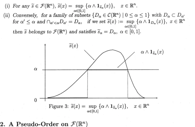
representative theorem (cf. [7, 10]).

(i) For any$\overline{s}\in \mathcal{F}(\mathbb{R}^{n}),$ $\overline{s}(X)=\sup$

{

$\alpha$A $1_{\overline{s}_{\alpha}}(x)$

},

$x\in \mathbb{R}^{n}$. $\alpha\in[0,1]$

(ii) Conversely, for

a

$f\mathrm{a}\mathrm{m}ily$ of$su$bsets $\{D_{\alpha}\in C(\mathbb{R}^{n})|0\leq\alpha\leq 1\}$ with $D_{\alpha}\subset D_{\alpha’}$

for $\alpha’\leq\alpha$ and $\bigcap_{\alpha’<\alpha}D_{\alpha^{J}}=D_{\alpha}$, if

we

set

$\overline{S}(X):=\sup_{\alpha\in[0,1]}$

{

$\alpha$ A $1_{D_{\alpha}}(x)$

},

$x\in \mathbb{R}^{n}$

then $\overline{s}$ belongs to _{$F(\mathbb{R}^{n})$} and

sa

tisfies $\overline{s}_{\alpha}=D_{\alpha},$ $\alpha\in[0,1]$.

2. A

Pseudo-Order

on

$\mathcal{F}(\mathbb{R}^{n})$

In this section,

we

review

a

pseudo order introduced by [7] and give a related result

necessary in the sequel. Henceforth

we

assume

that the

convex cone

$K\subset \mathbb{R}^{n}$ is given. A

pseudo order $\neg K\prec$

on

$C(\mathbb{R}^{n})$ is defined, whose idea is based

on a

set-relation treated in [8],

as follows.

For$A,$ $B\in C(\mathbb{R}^{n}),$ $A\neg\prec_{K}B\mathrm{m}e$

ans

the following (C.a) and (C.b) :

(C.a) For any $x\in A$, there exists $y\in B$ such that $x\prec_{\neg K}y$.

(C.b) For any$y\in B$, there exists $x\in A$ such that $x\neg\prec_{K}y$.

$A$

(C.a) (C.b)

When $K=\mathbb{R}_{+}^{n}$, the relation $\neg K\prec$

on

$C(\mathbb{R}^{n})$ will be written simply by $\neg n\prec$ with

some

abuse of notation and for $[x, y],$ $[x^{J\prime}, y]\in C_{r}(\mathbb{R}^{n}),$ $[x, y]\neg n\prec[x’, y]’$

means

$x\neg n\prec x’$ and $y\neg n\prec y’$. Note that $\neg n\prec$

on

$C(\mathbb{R}^{n})$ is partial order.

Using a pseudo order $\neg K\prec$ on $\mathbb{R}^{n}$,

a

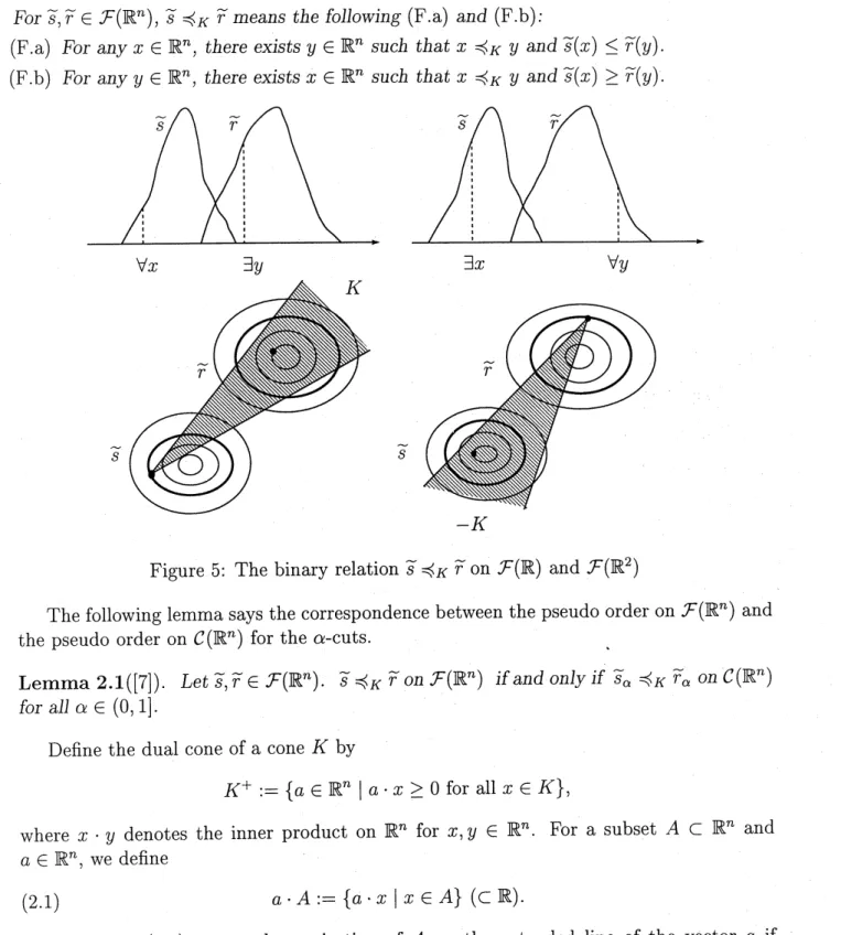
pseudo order $\neg K\prec$ on $F(\mathbb{R}^{n})$ is defined as follows.

$Forsr\sim,$$\sim\in F(\mathbb{R}^{n}),$ $\overline{s}\neg\prec_{K}\overline{r}$ me

ans

the followi$\mathrm{n}g$ (F.a) and (F.b):

(F.a) For any$x\in \mathbb{R}^{n}$, there exists $y\in \mathbb{R}^{n}$ such that $x\neg K\prec y$ an$d\overline{s}(x)\leq\overline{r}(y)$.

(F.b) For any $y\in \mathbb{R}^{n}$, there exists $x\in \mathbb{R}^{n}$ such that $x\neg K\prec y$ an$d_{S}^{\sim}(x)\geq\sim r(y)$.

$3x$ $\nabla y$

Figure 5: The binary relation $\overline{S}_{\neg K}\prec\overline{r}$

on

$\mathcal{F}(\mathbb{R})$ and $F(\mathbb{R}^{2})$

The following lemmasays the correspondence between the pseudo order on $\mathcal{F}(\mathbb{R}^{n})$ and

the pseudo order on $C(\mathbb{R}^{n})$ for the $\alpha$-cuts.

Lemma 2.1([7]). Let $\overline{s},$$\overline{\gamma}\in \mathcal{F}(\mathbb{R}^{n})$. $\overline{s}\neg\prec_{K}r\sim$

on

$\mathcal{F}(\mathbb{R}^{n})$ if and on$l\mathrm{y}$$i\mathrm{f}\sim s_{\alpha}\neg\prec_{K}\overline{r}_{\alpha}$on $C(\mathbb{R}^{n})$

for all $\alpha\in(0,1]$.

Define the dual

cone

of a

cone

$K$ by

$K^{+}.--$

{

$a\in \mathbb{R}^{n}|a\cdot x\geq 0$ for all $x\in K$

},

where $x\cdot y$ denotes the inner product on

$\mathbb{R}^{n}$ for

$x,$$y\in \mathbb{R}^{n}$. For a subset $A\subset \mathbb{R}^{n}$ and $a\in \mathbb{R}^{n}$, we define

(2.1) $a\cdot A:=\{a\cdot x|x\in \mathrm{A}\}(\subset \mathbb{R})$

The equation (2.1)

means

the projection of $A$

on

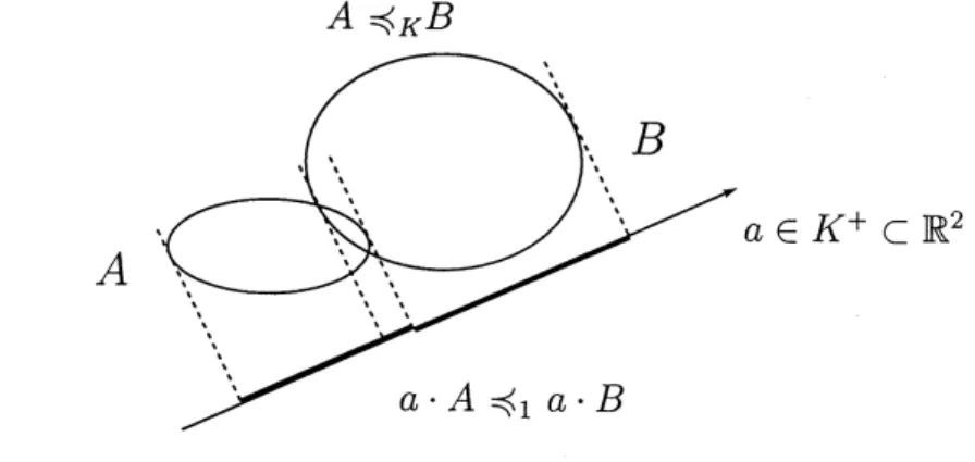
the extended line of the $\mathrm{v}e$ctor $a$ if

Lemma $2.2([7])$. Let $A,$$B\in C(\mathbb{R}^{n})$. $A\neg K\prec B$ on $C(\mathbb{R}^{n})$ if and only if $a\cdot A\neg 1\prec a\cdot B$ on

$C(\mathbb{R})$ for all$a\in K^{+}$.

$A\prec_{-\Gamma\nearrow}R$

$A$

Figure 6: The image ofLemma 2.2

For $a\in \mathbb{R}^{n}$ and $\overline{s}\in F(\mathbb{R}^{n})$, we define a fuzzy number $a\cdot s\sim\in \mathcal{F}(\mathbb{R})$ by

(2.2) $a \cdot\overline{s}(x):=\sup_{\alpha\in[0,1]}\mathrm{m}\mathrm{i}\mathrm{n}\mathrm{f}\alpha,$

$1a\cdot\overline{S}_{\alpha}(x)\}$, $x\in \mathbb{R}$.

The following theorem gives the correspondence between the pseudo-order $\neg K\prec$

on

$F(\mathbb{R}^{n})$ and the fuzzy _$\max$ order $\neg 1\prec$

on

$\mathcal{F}(\mathbb{R})$.

Lemma 2.3 ([7]). For $\overline{s},$$r\sim\in F(\mathbb{R}^{n}),$ $\overline{s}\neg\prec_{K}r\sim if$and onlyif $a\cdot s\neg\prec_{1}\sim a\cdot\overline{r}$ for all$a\in K^{+}$.

$a\cdot s\neg\prec_{1}a\cdot r$

Figure 7: The image of Lemma 2.3

A closed

cone

$K$ is said to be acute (cf. [12]) if there exists an $a\in \mathbb{R}^{n}$ such that

$a\cdot x>0$ for all $x\in K$ with $x\neq 0$. We have the following lemma.

Lemma 2.4. Let $K$ be a closed, $ac\mathrm{u}te$

convex

cone and _{$x_{0},$ $y_{0}\in \mathbb{R}^{n}$} with _{$x_{0}\prec_{\neg K}y_{0}$}.

Let $\rho$ be the Hausdorff metric on $C(\mathbb{R}^{n})$, that is, for $A,$ $B\in C(\mathbb{R}^{n}),$ $\rho(A, B)=$

$\max_{a\in A}d(a, B)\vee\max d(bb\in B’ A)$, where $d$is a metric in $\mathbb{R}^{n}$ and

$d(x, Y)= \min_{y\in Y}d(x, y)$ for $x\in \mathbb{R}^{n}$

and $Y\in C(\mathbb{R}^{n})$. It is well-known that $(C(\mathbb{R}^{n}), \rho)$ is a complete metric space. A sequence $\{D\ell\}_{\ell=1}^{\infty}\subset C(\mathbb{R}^{n})$ converges to $D\in C(\mathbb{R}^{n})$ w.r.t. $\rho$ if$\rho(D_{\ell}, D)arrow \mathrm{O}$ as $parrow\infty$.

Definition(Convergence offuzzy set, [17]).

For $\{\overline{s}_{l}\}_{\ell}\infty=1\subset F(\mathbb{R}^{n})$ and $\overline{r}\in \mathcal{F}(\mathbb{R}^{n}),\overline{s_{l}}$

converges

to $\overline{r}W.r.t$

.

$\rho$ if $\rho(\overline{s}_{f\alpha},, \overline{r}_{\alpha})arrow 0$

as

$\ellarrow\infty$ except at $\mathrm{m}ost$ countable $\alpha\in[0,1]$.

3. Sequences

in

$C(\mathbb{R}^{n})$

In this section, restricting $C(\mathbb{R}^{n})$ into the subclass by

use

of the concept of determining

class,

we

prove the monotone convergence theorem.

Let $K$ be a convex

cone.

The sequence $\{D_{f}\}_{\ell}\infty=1\subset C(\mathbb{R}^{n})$ is said to be bounded w.r.t.

$\prec_{\neg K}$ ifthere exists $F,$$D\in C(\mathbb{R}^{n})$ such that $F\neg K\prec D_{f}\neg K\prec D$ for all $\ell\geq 1$ and said to be

monotone w.r.t. $\neg K\prec$ if$D_{1}\neg K\prec D_{2}\neg K\prec\ldots$

.

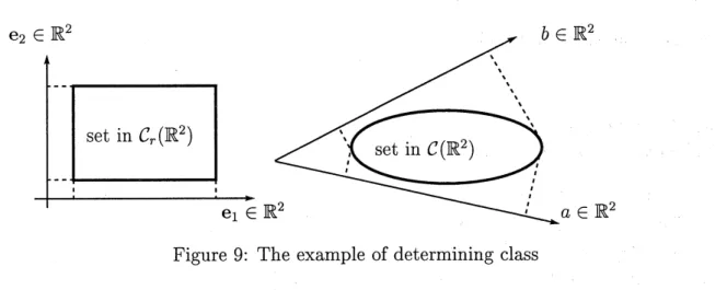
Let $L\subset C(\mathbb{R}^{n})$ and $A\subset \mathbb{R}^{n}$. Then we say that $A$ is a determining class for $L$ if $a\cdot D=a$ , $F$ for all $a\in A$ and $D,$$F\in,\mathbb{C}$ implies $D=F$. For example, the set of unit

vectors $\{\mathrm{e}_{1}, \mathrm{e}_{2}, , . . , \mathrm{e}_{n}\}$ in $\mathbb{R}^{n}$ is

a

determining class for $C_{r}(\mathbb{R}^{n})$. Also, by the separation

theorem, $\mathbb{R}^{n}$ is a determining class for $C(\mathbb{R}^{n})$.

Figure 9: The example of determining class

Theorem 3.1. Let $K$ bea closed convex cone of$\mathbb{R}^{n}$. Suppose that $K^{+}$ is a determining

classfor $L\subset C(\mathbb{R}^{n})$. Then, the pseudo order $\neg K\prec$ becomes a$p$arti$\mathrm{a}l$ order in the restricted

class L.

As a simple application of Theorem 3.1, we have the following.

Corollary 3.1. Let $K$ be

a

closed

convex cone

of$\mathbb{R}^{n}$ and _{$L\subset C(\mathbb{R}^{n})$} closed. Suppose

that $K^{+}$ is a determining class for L. Then, any sequen

ce

$\{D_{l}\}\subset L$ which is $\mathrm{m}$onotone

$w.r.t$. $\neg K\prec$ and satisfies $D_{l}\subset X(l\geq 1)$ for

some

compact subset$X$ of

$\mathbb{R}^{n}$ converges $w.r.t$.

$\rho$.

In order to continue a further discussion, we need the acuteness of the ordering cone

We have the following.

Lemma3.1. Let$K$ be

a

closed, acute

convex

cone

and$D,$$F,$ $G\in C(\mathbb{R}^{n})$ with$D\prec F\prec G\neg K\neg K$.

Let (3.1)

$X:=x \in D\bigcup_{x\prec_{Ky}\neg},y\in G(x+K)\cap(y-K)$

.

Then, it holds that $F\subset X$ and $X$ is bounded.

Theorem 3.2. Let $K$ be a closed, $ac\mathrm{u}te$

convex

cone of $\mathbb{R}^{n}$ and _{$L\subset C(\mathbb{R}^{n})$} closed.

Suppose that $K^{+}$ is a determining class for L. Then, any seq$\mathrm{u}$ence $\{D_{l}\}^{\infty}\iota=1\subset L$ which is

bounded and $\mathrm{m}$onotone $w.\mathrm{r}.6$. $\neg K\prec$

converges

$w.r.t$. $\rho$.

As applications of Theorem 3.2, we have the following Corollaries.

Corollary 3.3. Anysequ

ence

in $C_{r}(\mathbb{R}^{n})$ with $\mathrm{m}$onotonicity and boundedness $w.\mathrm{r}.t$. $\neg n\prec$

converges $w.r.t$. $\rho$.

For any $D\in C(\mathbb{R}^{n})$ and $\xi>0$, the $\epsilon$-closed neighborhood of$D$ will be denoted by

(3.2) $S_{\epsilon}(D):=\{x\in \mathbb{R}^{n}|d(x, D)\leq\in\}$,

which is

a

compact

convex

subset of$\mathbb{R}^{n}$. Note that

(3.3) $s_{\epsilon}(D)=D+\xi U0$,

where $U_{0}$ is the closed unit ball (cf. [2]).

The following lemma is useful in the sequel. Lemma 3.2. The following (i) to (iii) hold.

(i) For any $D,$$F\in C(\mathbb{R}^{n})$, if$S_{\delta_{1}}(D)\subset S_{\delta_{2}}(F)$ for

some

$\delta_{1},$$\delta_{2}\geq 0$,

then $S_{\delta_{1}+\mathit{6}}(D)\subset S_{\delta_{2}+\epsilon}(F)$ for any$\epsilon\geq 0$.

(ii) For any $D\in C(\mathbb{R}^{n})$ and $\lambda>0,$ $S_{\xi}i(\lambda D)=\lambda s_{/\lambda}\epsilon(D)$.

(iii) For any sequence $\{D_{l}\}\subset C(\mathbb{R}^{n})$ and $D\in C(\mathbb{R}^{n})$, if$D_{l}arrow D$

as

$larrow\infty$,

then $S_{\delta}(D_{\iota)}arrow S_{\delta}(D)$

as

$larrow\infty(\delta\geq 0)$.

For any closed

convex cone

$K\subset \mathbb{R}^{n}$, let $L(K^{+})$ be the set of all $D\in C(\mathbb{R}^{n})$ satisfying

that for any $x_{0}\in \mathbb{R}^{n}$ and $\epsilon>0$ with $x_{0}\not\in S_{\epsilon}(D)$ there exists $a\in K^{+}(a\neq 0)$ such that

$a\cdot y\geq a\cdot x_{0}$ for all $y\in S_{\epsilon}(D)$.

The properties of$L(K^{+})$

are

stated in the following lemma.

Lemma 3.3. The following (i) to (iii) hold.

(i) $K^{+}$ is a determiningclass for $L(K^{+})$.

(iii) For any $D\in L(K^{+}),$ $\lambda D+\mu D\in \mathcal{L}(K^{+})(\lambda, \mu\geq 0)$.

Noting that $K^{+}=\mathbb{R}_{+}^{2}$ when $K=\mathbb{R}_{+}^{2}$ in $\mathbb{R}^{2}$, the

sets included in $L(\mathbb{R}_{+}^{2})$ are illustrated

in Figure 10.

Theorem 3.3. Let $K$ be

a

closed, acute

convex

cone

of $\mathbb{R}^{n}$. Then, any sequence

$\{D_{l}\}^{\infty}\iota=1\subset L(K^{+})$ which is bounded and $\mathrm{m}$onotone $w.r.t$. $\neg K\prec$ converges $w.r.t$. $\rho$.

4. Sequences

in

$\mathcal{F}(\mathbb{R}^{n})$

In this section, the monotone convergence theorem for

a

sequence in $\mathcal{F}(\mathbb{R}^{n})-$ is given.

Let $\overline{L}\subset \mathcal{F}(\mathbb{R}^{n})$ and $A\subset \mathbb{R}^{n}$. Then we call $A$ a determining class for _,$\mathrm{C}$ if $a\cdot\overline{s}=a\cdot\overline{r}$

for all $a\in A$ and $\overline{s},$

$r\sim\in,\sim \mathrm{C}$

implies $\overline{s}=\overline{r}$.

A natural extension of Theorem 3.1 to fuzzy sets will be given in the following theorem.

Theorem 4.1. Let $K$ be a closed convex

cone

of$\mathbb{R}^{n}$ and $\overline{L}\subset F(\mathbb{R}^{n})$.

$S\mathrm{u}p\underline{p}oSe$ that $K^{+}$

$is$ a determining $cl\mathrm{a}SS$ for $\overline{L}$

. Then, a pseudo order $\neg\prec K$ is a partial order in $L$.

Let $K$ be

a

convex

cone. The sequence $\{\overline{s}_{l}\}\subset F(\mathbb{R}^{n})$ is said to be bounded w.r.t. $\neg K\prec$

if there $\mathrm{e}\mathrm{x}\mathrm{i}_{\mathrm{S}}\mathrm{t}_{\mathrm{S}u},$$\overline{v}\sim\in F(\mathbb{R}^{n})$ such that $\overline{u}\neg\prec_{K}s_{\iota}\sim\neg\prec_{K}\overline{v}\mathrm{f}_{0}\mathrm{r}$all $l\geq 1$ and said to be monotone

w.r.t.

$..$

$\neg K\prec$ if$\overline{s}_{1}\neg K\prec\overline{s}_{2}\neg K\prec\ldots$

.

In order to obtain theconvergence theorem,

we

need the concept of directionality given

in [17]. Denote thesurface of the unit ball by $U:=\{x\in \mathbb{R}^{n}|||x||=1\}$. Let $V\subset U$. Then,

for $D,$$D’\in C(\mathbb{R}^{n})$ with $D\subset D’$, we call $D’V$-directional to $D$ (written by $D’\supset_{V}D$) if

there exists

a

real $\lambda>0,$$y\in D$ and $z\in D’$ such that

(i) $d(z, y)=\rho(D’, D)$ and (ii) $z-y=\lambda v$ for

some

$v\in V$_.

Definition (V-directional). Let $V\subset \mathbb{R}^{n}.$ For$\overline{s}\in F(\mathbb{R}^{n}),$ $\overline{s}$ is called

$V$-direction$\mathrm{a}l$ if

$\sim s_{\alpha}\supset_{V}\overline{s}_{\alpha}$_; for $0\leq\alpha\leq\alpha’\leq 1$.

Corollary 4.1. Let $K$ be a closed $con$vex cone of$\mathbb{R}^{n}$ and $\tilde{L}\subset F(\mathbb{R}^{n})$ closed. Suppose

that $K^{+}$ is a determining $cl\mathrm{a}SS$ for $\overline{L}$

. Let a sequence $\{\overline{s}_{l}\}\subset F(\mathbb{R}^{n})$ be satisfied that

(b) $each_{\overline{S}}\iota$ is $V$-directional for

a

finite set $V\subset \mathbb{R}^{n}$ and

(c) there exists a compact subset $D$ of$\mathbb{R}^{n}$ such that $\overline{s}\iota 0\subset D$ for all $l\geq 1,$ where $\overline{s}_{l0}$ is

the support or the $0$-cut $of\overline{s}_{l}$.

Then the sequence $\{\overline{s}_{l}\}$ converges $w.r.t$. $\rho$.

The following monotoneconvergence theorem is thought of

as an

extension of Theorem

3.2 to fuzzy sets.

Theorem 4.2. Let $K$ be a closed, acute

convex cone

of$\mathbb{R}^{n}$ and $\overline{L}\subset \mathcal{F}(\mathbb{R}^{n})$ closed.

Suppose that $K^{+}$ is a determining class for $\overline{L}$

closed. Then, any sequence $\{\overline{s}_{\iota\}_{l}^{\infty}}=1\subset\overline{L}$

which satisfies (a) and $(b)$ in Corollary 4.1 converges $w.r.t$. $\rho$.

Now, for any closed

convex cone

$K$, we define $\overline{L}(K^{+})$ by

$\overline{L}(K^{+}):=$

{

$\overline{s}\in \mathcal{F}(\mathbb{R}^{n})|s_{\alpha}\sim\in L(K^{+})$ for all $\alpha\in[0,1]$

}.

The previous Lemma 3.3 is extended to that for $\mathcal{F}(\mathbb{R}^{n})$ in the following lemma.

Lemma 4.1. The following (i) to (iii) hold. (i) $K^{+}$ is a determining class for $\overline{L}(K^{+})$.

(ii) $\overline{L}(K^{+})$ is closed $w.r.t$. the convergence defined in Section 2.

(iii) For any $\overline{s}\in\overline{L}(K^{+}),$ $\lambda\overline{s}+\mu\overline{s}\in\overline{L}(K^{+})(\lambda, \mu\geq 0)$.

We have the following.

Theorem 4.3. Let $K^{+}$ be

a

closed, acute

convex cone

of$\mathbb{R}^{n}$. Then, any sequ

ence

$\{\overline{s_{l}}\}_{l1}\infty=\subset\overline{L}(K^{+})$ which

sa

tisfies (a) and (b) in Corollary 4.1 converges.

5. Applications to Monotone Dynamic

Fuzzy Systems

In this section,

as

an application of the results obtained in the preceding section, we

consider

a

limit theorem for

a

sequence of fuzzy states defined by the dynamic fuzzy

system (cf. [5, 6, 14, 15, 16, 17]) with

a

monotone fuzzy relation.

Let $\overline{q}:\mathbb{R}^{n}\cross \mathbb{R}^{n}arrow[0,1]$ be

a

continuous fuzzy relation such that $\overline{q}(x, \cdot)\in F(\mathbb{R}^{n})$ for

each $x\in \mathbb{R}^{n}$ and

$q$

is convex, that is,

(5.1) $\overline{q}(\lambda X^{1}+(1-\lambda)X^{2}, \lambda y^{1}+(1-\lambda)y)2\geq\overline{q}(x^{1}, y^{1})$ A $\overline{q}(x^{2}, y^{2})$

for any $x^{1},$ $x^{2},$ $y^{1},$ $y^{2}\in \mathbb{R}^{n}$ and $\lambda\in[0,1]$. From this fuzzy relation $\overline{q}$, we define $\overline{q}:F(\mathbb{R}^{n})arrow$

{the

set of fuzzy sets on $\mathbb{R}^{n}$

}

as follows.

(5.2) $\overline{q}(\overline{u})(y)$

$:= \sup_{\mathbb{R}^{n}x\in}$

{

$\overline{u}(_{X)}$ A $\overline{q}(x,$$y)$

}

$,$

$\in \mathbb{R}^{n}$,

where $a$ A $b= \min\{a, b\}$. Also, for any $\alpha\in[0,1],\overline{q}_{\alpha}$ :

$C(\mathbb{R}^{n})arrow 2^{\mathbb{R}^{n}}$ will be defined by

(5.3) $\overline{q}_{\alpha}(D):=\{$

{

$y|\overline{q}(x,$$y)\geq\alpha$ for

some

$x\in D$

},

for $\alpha>0,$ $D\in C(\mathbb{R}^{n})$ $\mathrm{c}1$

{

$y|\overline{q}(x,$ $y)>0$ for

some

$x\in D$

},

for $\alpha=0,$ $D\in C(\mathbb{R}^{n})$,

where cl denotes the closure of a set and $2^{\mathbb{R}^{n}}$

the set of all closed subsets of $\mathbb{R}^{n}$. For

simplicity, we put $q(\sim x):=\overline{q}(\{x\})$ for $x\in \mathbb{R}^{n}$.

The following facts are well-known (cf. [4, 5, 17]).

Lemma 5.1 The following (i) to (iii) hold.

(i) $\overline{q}_{\alpha}(D)\in C(\mathbb{R}^{n})$ for any$D\in C(\mathbb{R}^{n})$ and$\overline{q}_{\alpha}(\cdot)$ is contin

uous

in$C(\mathbb{R}^{n})$ for each $\alpha\in(0,1]$. (ii) $\overline{q}(\overline{u})\in F(\mathbb{R}^{n})$ for any $\overline{u}\in F(\mathbb{R}^{n})$.

(iii) $\overline{q}(\overline{u})_{\alpha}=q_{\alpha}(\sim\overline{u})_{\alpha}$ for any$u\sim\in \mathcal{F}(\mathbb{R}^{n})$ and $\alpha\in[0,1]$, where $\overline{q}(\overline{u})_{\alpha}$ is the $\alpha$-cut of$q(\sim\overline{u})$.

The sequence of fuzzy states, $\{\overline{s}_{t}\}_{t=1}^{\infty}\subset F(\mathbb{R}^{n})$, for the dynamic system with fuzzy

transition $\overline{q}$is defined

as

follows.

(5.4) $\sim_{\iota+1\overline{q}(}s=\overline{S}_{t})$ $(t\geq 1)$,

where $\overline{S}_{1}\in \mathcal{F}(\mathbb{R}^{n})$ is the initial fuzzy state.

The problem in this section is to consider a convergence of the sequence $\{s_{t}\}_{t=1}^{\infty}\sim$ defined

by (5.4),

so

that

we

derive the monotone property ofthe fuzzy relation $\overline{q}\mathrm{w}.\mathrm{r}.\mathrm{t}$. the pseudo

order $\neg\prec K$ defined by the ordering

cone

$K$ in $\mathbb{R}^{n}$.

Definition ($\neg\prec_{K}$-monotone). The fuzzy relation $\overline{q}$is called

$\neg K\prec$-monotone

if $x^{1}\prec_{\neg K}x^{2}$ $(x^{1}, x^{2}\in \mathbb{R}^{n})$

means

$q(\sim x^{1}, \cdot)\neg K\prec\overline{q}(x^{2}, \cdot)$.

Remark. Yoshida et al [17] has introduced

a

monotone property concerning the fuzzy

relation $\overline{q}\mathrm{w}\mathrm{h}\mathrm{o}\mathrm{S}\mathrm{e}$ definition is

as

follows: $\overline{q}_{\alpha}(y)\subset q_{\alpha}(\sim x)+\ell(x, y)$ for

$x,$$y\in \mathbb{R}^{n}$, where

$\ell(x, y):=\{\gamma(y-x)|\gamma\geq 0\}$. Obviously, if$\overline{q}$is monotone in the

sense

of [17], then $\overline{q}$is

$\neg n\prec$-monotone, but the

converse

is not necessarily true.

The following lemma is useful for

our

further discussion.

Lemma 5.2. Suppose that $q\prec\sim_{i\mathrm{s}_{\neg K}}$-monotone. Then, for

$a,n.yu,$$\overline{v}\sim\in F(\mathbb{R}^{n})$ with

$\overline{u}\neg\prec_{K}\overline{v}$,

it holds that $\overline{q}(u)\sim\neg K\prec\overline{q}(v)\sim$.

Assumption A. The following (i) to (iii) hold.

(i) The $ord$eringcone $K$ is

a

$cloSed$, acute

convex

one in $\mathbb{R}^{n}$.

(ii) The fuzzy$rel$ation $qis\sim\prec_{\neg K}$-monotone.

(iii) There exists a finite subset $V\subset U$ such that, for any $D,$ $D’\in C(\mathbb{R}^{n})(D’\supset D)$, if

$D’\supset_{V}D$ then $\overline{q}_{\alpha’}(D’)\supset_{V\overline{q}_{\alpha}}(D)$ for all $\alpha,$ $\alpha’(0\leq\alpha’\leq\alpha\leq 1)$.

1 ,$\cdot$ . .

For any given $\overline{u}\in F(\mathbb{R}^{n}),$ putting $\overline{s}_{1}:=\overline{u}$,

we

define the sequence $\{s_{t}\}_{t=1}^{\infty}\sim$ by (5.4).

Then,

we

have the following.

Theorem 5.1. In addition to Assumption $A$, suppose that the following (iv) to (vi) hold.

(iv) $\overline{u}\in\overline{L}(K^{+})$ and $\overline{u}\neg\prec_{K}\overline{q}(\overline{u})$.

(vi) $\{s_{t}\}\sim\subset\tilde{L}(K^{+})$ and bounded from above.

Then, thesequence$\{\overline{s}_{t}\}$ converges andthe limit $\overline{s}:=\lim_{tarrow\infty^{S_{l}}}\sim$

sa

tisfies the following fuzzy

$rel$

a

tion$\mathrm{a}l$ equation:

(5.5) $\sim\sim s=q(\overline{s})$.

Theorem 5.2. In addition to Assumption $A$, suppose that the following $(\mathrm{i}\mathrm{v}’),$ $(\mathrm{v})$ an$d$

$(\mathrm{v}\mathrm{i}’)$ hold.

$(\mathrm{i}\mathrm{v}’)u\sim\in\overline{L}(K^{+})$ with $u_{0}\sim\subset K$ and $\overline{q}(\overline{u})\neg\prec_{K}\overline{u}$.

(v) $\overline{u}_{\alpha’}\supset_{V}q_{\alpha}\sim$ for all

$\alpha,$$\alpha’(0\leq\alpha’\leq\alpha\leq 1))$, where $V$ is as in Assumption A(iii).

$(\mathrm{v}\mathrm{i}’)$

. $\{\overline{S}_{t}\}\subset\tilde{L}(K^{+})$.

Then, the sequence$\{\overline{s}_{t}\}$ convergesand the$limit \overline{s}:=\lim_{tarrow\infty^{\overline{S}}t}$

sa

tisfies the fuzzy_$rel$ation$\mathrm{a}l$

equation (5.5).

As

an

example of $\neg K\prec$-monotone fuzzy relation, we put the fuzzy relation $\overline{q}$by

(5.6) $\overline{q}(x, y):=r(\sim y)+\beta 1_{\{\}}x$ $(x, y\in \mathbb{R}^{n})$,

$\mathrm{w}\mathrm{h}\mathrm{e}\mathrm{r}\mathrm{e}\sim r\in\overline{L}(K^{+})$ with $\overline{r}_{\alpha’}\supset_{V}\overline{r}_{\alpha}$ for

some

finite set $V\subset U$ and

$\alpha,$$\alpha’(0\leq\alpha’\leq\alpha\leq 1)$

and $0<\beta<1$.

Obviously, Assumption A is satisfies for $q\mathrm{o}\mathrm{f}\sim(5.6)$. Also, we observe from Lemma 4.1

that the assumptions (iv) to (vi) in Theorem 5.1 hold $\mathrm{f}\mathrm{o}\mathrm{r}u\sim=\overline{r}$. So that by Theorem 5.1,

the sequence $\{\overline{s}_{t}\}$ defined by (5.4) $\mathrm{w}\mathrm{i}\mathrm{t}\mathrm{h}_{\overline{S}_{1}}=\sim r$converges.

Remark. Note that the fuzzy relation $q\mathrm{o}\mathrm{f}\sim(5.6)$ satisfies the contraction property

intro-duced in [4]. Thus,

we see

that the limit $\overline{s}=\lim_{tarrow\infty^{s_{t}}}\sim$ is

a

unique solution of the fuzzy

relational equation (5.5) and given $\mathrm{b}\mathrm{y}s\sim=(1-\beta)^{-1}\overline{r}$.

Example. We give

a

one-dimensional numerical example whose fuzzy relation $\overline{q}$is given

by

$\overline{q}(x, y)=(1-2|y-(3-X^{-2})|)\vee 0$ _$(x>0)$.

For $\alpha\in[0,1]$, it holds that by (5.3)

$\overline{q}_{\alpha}(x)=[3-(1-\alpha)2-1-x-2,3+(1-\alpha)2^{-1}-X^{-2}]$_.

This is illustrated in Figure 2. So,

we

observe that $\overline{q}$is $\prec_{\neg 1}$-monotone in $(0, \infty)\cross(0, \infty)$,

also that $1_{\{1\}}\neg\prec 1\overline{q}(1_{i}1\})$ and $\overline{q}(x, \cdot)\neg 1\prec 1_{\{7/2\}(x})$.

Applying Theorem 5.1, the sequence $\{\overline{s}_{t}(X)\}$ defined by (5.4) with _{$\sim s_{1}(x)=1_{\{1\}}(x)$}

converges. The

convergence

is shown in Figure 2 and 3 with the limit $\overline{s}(X)=\lim_{tarrow\infty}S_{t}(\sim)X$,

where the $\alpha$-cut $\sim s_{\alpha}$ of the limit $\overline{s}(x)$ for $\alpha=0$ and $\alpha=1$

are

$\min\overline{s}_{0}=$ 2.313099034,

Figure 11: $q_{\alpha}(\sim x)$ and the limit $\overline{s}(X)$ of $\{\overline{s}_{t}(X)\}$

Figure 12: The sequence $\{\overline{s}_{t}(X)\}$

References

[1] W.Congxin and C.Cong, “The supremum and infimum of the set of fuzzy numbers

[2] P.Diamond and P.Kloeden, Metric Spaces

_of

Fuzzy $Sets_{\mathrm{z}}$ Theory and Applications

(World Scientific, 1994).

[3] N.Furukawa, “Parametric orders

on

fuzzy numbers and their roles in fuzzy

optimiza-tion problems,” Optimization 40 (1997) 171-192.

[4] M.Kurano, M.Yasuda, J.Nakagami andY.Yoshida, “A limittheorem insome dynamic

fuzzy systems,” Fuzzy Sets and Systems 51 (1992) 83-88.

[5] M.Kurano, M.Yasuda, J.Nakagami and Y.Yoshida, “Markov-type fuzzy decision

pro-cesses

with

a

discounted reward on a closedinterval,” European Journal

_of

Operations

Research 92 (1996)

649-662.

[6] M.Kurano, M.Yasuda, J.Nakagami and Y.Yoshida, “The time average reward for

some dynamic fuzzy systems,” Computers and Mathematics with Applications 37

(1999) 77-86.

[7] M.Kurano, M.Yasuda, J.Nakagami and Y.Yoshida, “Ordering of fuzzy sets–A brief

survey and new results,” J. Operations Research Society

_of

Japan 43 No.l (2000)

138-148.

[8] D.Kuroiwa, T.Tanaka and T.X.D.Ha, “On

cone

convexity of set-valued maps,”

Non-linear Analysis, Theory $\xi y$ Applications 30 (1997) 1487-1496.

[9] Nanda,S., $‘\zeta \mathrm{O}\mathrm{n}$ sequences of fuzzy numbers”, Fuzzy Sets and Systems 33 (1989)

123-126.

[10] V.Nov\’ak, Fuzzy Sets and Their Applications (Adam Hilder, Bristol-Boston, 1989).

[11] J.Ram\’ik and

J.\v{R}im\’anek,

“Inequality relation between fuzzy numbers and its use in

fuzzy optimization,” Fuzzy Sets and Systems 16 (1985) 123-138.

[12] J.Stoer and C.Witzgall, Convexity and Optimization in Finite Dimensions $I$

(Springer-Verlag, Berlin and New York, 1970).

[13] Y.R.Syau, “Sequences in

a

fuzzy metric space,” Computers and Mathematics with

Applications 33 (1997) 73-76.

[14] Y.Yoshida, M.Yasuda, J.Nakagami and M.Kurano, “A potential of fuzzy relations

with a linear structure: The contractive case,” Fuzzy sets and Systems 60 (1993)

283-294.

[15] Y.Yoshida, M.Yasuda, J.Nakagami and $\mathrm{M}.\mathrm{K}\mathrm{u}\mathrm{r}\mathrm{a}\mathrm{n}\mathrm{o}$

)”

“A potential of fuzzy relations

with a linear structure: The unbounded case, Fuzzy sets and Systems 66 (1994)

83-96.

[16] Y.Yoshida, “A time-average fuzzy reward criterion in fuzzy decision processes,)’

In-formation

Sci. 110 (1998) 103-112.

[17] Y.Yoshida, M.Yasuda, J.Nakagami and M.Kurano, “A limit theorem in dynamic fuzzy

systems with a monotone property,” Fuzzy sets and Systems 94 (1998) 109-119.

[18] L.A.Zadeh, “Fuzzy sets,”

_Inform.

and Control 8 (1965) 338-353.

[19] K.Zhang and K.Hirota, “On fuzzy number lattice $(\tilde{R}, \neg\prec),’)$ Fuzzy sets and Systems