九州大学学術情報リポジトリ
Kyushu University Institutional Repository
プローブデータを利用した隣接バス停間の移動時間 予測に関する研究
マンスル, アス
http://hdl.handle.net/2324/2236255
出版情報:Kyushu University, 2018, 博士(工学), 課程博士 バージョン:
権利関係:
GRADUATE SCHOOL OF INFORMATION SCIENCE AND ELECTRICAL ENGINEERING
A Study on Prediction of Travel Time over Intervals between Adjacent Bus Stops Using Probe Data
Author:
Mansur As
Supervisor:
Professor Tsunenori Mine
A thesis submitted in partial fulfillment of the requirements for the degree of Doctor of Engineering (Computer Science)
in the
DEPARTMENT OF ADVANCED INFORMATION TECHNOLOGY
Japan
January 25, 2019
Abstract
Mansur As
A Study on Prediction of Travel Time over Intervals between Adjacent Bus Stops Using Probe Data
Prediction of travel time over travel routes is an important factor for many people who travel or commute, especially using the public bus services. Mostly, people consider travel time as well as stochastic factors in several time peri- ods such as dwell time, traffic congestion, accidents, and so on. They usually prefer to minimize the time spent traveling from their origin to destination by choosing the best route. Intelligent Transportation Systems (ITSs) have re- cently been widely used in planning, evaluation and control of the reliability of the public transportation system. One of the evolutions in ITSs is largely related to bus probe data. Probe data, which are generated by vehicles, in- clude data obtainable from navigation systems, such as time and position (longitude and latitude), i.e. data on the vehicle’s running and performance history. In addition, using bus probe data enables us to monitor the state of road traffic characteristics and to measure the reliability of and variability in travel times of public bus services.
In this research, I have proposed nonlinear dynamical methods for pre- dicting bus travel time over each interval between adjacent bus stops for seven and eight time periods in a day. The proposed methods basically uti- lize time series methods based on machine learning techniques: Artificial
iv
Neural Network (ANN), Support Vector Machine (SVM) and Random For- est (RF). For this purpose, at first, I classified intervals between adjacent bus stops into two classes: stable and unstable. Then I identified two statistically significant factors: variabilities in travel time in the same time periods over days and correlations of travel time between eight time periods, which in- fluence bus travel time over unstable intervals in the current time period. I conducted experiments to evaluate our proposed methods. I have used real bus probe data collected from November 21st to December 20th, 2013 and provided by Nishitetsu Bus Company, Fukuoka, Japan. I summarize the re- sults obtained in this research as follows:
• Chapter 1 describes background information concerning Intelligent Trans- portation System (ITSs), including Bus Probe Data as a robust data source for predicting bus travel time, problem formulation, uniqueness of this research, the framework and the objectives of this research.
• Chapter 2 presents a literature review regarding prediction of bus travel time. A variety of models and algorithms have been developed to pre- dict bus arrival times or bus travel times, and these can be classified into the following categories: historical average models, regression/time se- ries models, and machine learning techniques including Artificial Neu- ral Network (ANN) Support Vector Machine (SVM) and Random For- est (RF).
• Chapter 3 explains the data used in this research, describes the prelim- inary data preparation for the analyses and the methods used in pre- diction models. In addition, I describe how real-world bus probe data can be utilized, what kind of analytic results are obtained, how the data should be calculated and what kind of challenges are involved when handling this bus probe data.
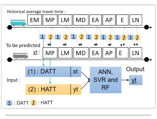
• Chapter 4 discusses some of the highlighted analytic results generated from the probe data. I first calculated the bus travel time over each interval between adjacent bus stops. Then, I distinguished the inter- vals into stable or unstable ones. Next, I conducted statistical analysis on travel time especially over unstable intervals considering the varia- tions in the travel time between different time periods in a day, in the same time periods over the past days and the correlation of travel time between adjacent time periods in a day. Based on the results of these analyses, I employed two types of input data: Dynamic Average Travel Time (DATT) and Historical average travel time (HATT). DATT denotes the average travel time in the time period right before the current one.
Introducing DATT can be expected to adjust the error in predicting travel time in the current time period using the travel time observed in the period just before the current time period. HATT denotes the av- erage travel time in the same time period during the past several days.
It is a very important input variable of the model because HATT is more effective when travel time tends to be more consistent over days.
• Chapter 5 proposes nonlinear dynamical models for predicting bus travel times using historical information. I developed time series prediction models based on Artificial Neural Network (ANN), Support Vector Ma- chine (SVM) and Random Forest (RF) to predict travel time over unsta- ble intervals. Focusing on recurrent and non-recurrent variabilities in travel time over the unstable intervals, I predicted travel time for seven time periods in a day (omitting EM) and compared the experimental results of the various approaches.
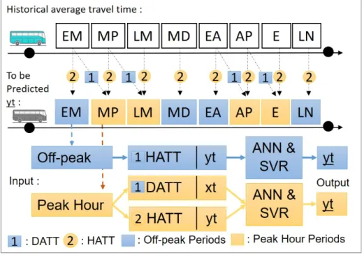
• Chapter 6 proposes a different approach for predicting bus travel time considering traffic congestion. This approach uses two input variables,
vi
DATT and HATT, selectively with a distinction between peak-hour and off-peak periods.
• Chapter 7 defines the role of these approaches in the evaluation of the performance of the prediction models. I compare the proposed model mentioned in Chapter 6 with the model mentioned in Chapter 5. In addition, to measure the significant effects of variables other than the single independent variable, I conduct an experiment comparing our models and the model proposed by another study.
• Finally, I conclude the thesis in Chapter 8. I describe the results of ex- periments and the findings of this research, and discuss some topics for future scientific research in the prediction bus travel time.
Acknowledgements
First of all, syukran wal hamdulillah thanks to Allah Subhana Wataalah, who gave me the strength and knowledge to accomplish this work.
I would like to express my deepest appreciation toProfessor Tsunenori Mine, for the crucial and patient help provided in developing this study. Most of this work was developed thanks to challenging objectives that he set through- out my research. Without his knowledge, patience, and support this disser- tation would not have been possible. The knowledge I gained from him will definitely influence the rest of my life. I am incredibly fortunate to have had him as an advisory under his tutelage and diligence all these years.
I would like to thank also Professor Akira Fukuda and Professor Kenji Hisazumi, as advisory committee members, for their comments and sugges- tions feedback were valuable in my PhD thesis.
I thank my friendDr. Eng. Nakamura Hiroyoki, first year in computer sci- ence, for his guidance for preparation bus probe data at the beginning of this study.
Sincere thanks to all laboratory members especially,Ms. Aya Miura, Mr. Ko- hei Yamaguchi, and Mr. Tsubasa Yamagucifor their help in the laboratory during my PhD study with their loving support, understanding and encour- agement.
viii
Thanks to the Nishitetsu Bus Company Fukuoka Japan, for providing the bus probe data for this research project.
At the end, I must offer my deep gratitude to my parents, brothers and my sister for their unconditional support during my study abroad. They have always been my source of enthusiasm. Special thanks to my wife and my son who enriched me with love, strength, and motivation.
Contents
Abstract iii
Acknowledgements vii
1 Introduction 1
1.1 Background . . . 1
1.2 Problem Formulation . . . 3
1.3 Uniqueness of this Research . . . 4
1.4 Research Objective and Scope . . . 5
1.5 Research Framework . . . 6
1.6 Research Question . . . 8
1.7 Contributions . . . 9
1.8 Thesis Outline . . . 10
2 Related Work 13 2.1 Introduction . . . 13
2.2 Travel Time Variability . . . 13
2.3 Methodology of Travel Time Prediction . . . 14
2.3.1 Historical Average Model with Time Series Approach . 15 2.3.2 Machine Learning Techniques . . . 17
2.4 Summary . . . 18
3 Data and Methodologies 21 3.1 Introduction . . . 21
3.2 Probe Data . . . 21
x
3.2.1 Overview . . . 21
3.2.2 Bus Probe Data . . . 22
3.3 Methodologies. . . 24
3.3.1 Travel Time over Intervals . . . 24
3.3.2 Distinguishing Stable and Unstable Intervals . . . 26
3.4 Methods of Travel Time Prediction . . . 29
3.4.1 Time Series Approach . . . 29
3.4.2 Artificial Neural Network (ANN) . . . 30
3.4.3 Support Vector Machine Regression (SVR) . . . 31
3.4.4 Random Forest (RF) . . . 33
3.4.5 Measures of Model Performance and Prediction Results 35 4 Preliminaries to Model Development 37 4.1 Introduction . . . 37
4.2 Travel Time Pattern Analysis . . . 38
4.3 Empirical Study on the Travel Time Variability . . . 41
4.4 Stable and Unstable intervals . . . 43
4.5 Travel Time Variation over Unstable Intervals . . . 45
4.5.1 Variability of Bus Travel Time between Time Periods . 45 4.5.2 Variability of Travel Time over Unstable Intervals In Each Time Period over Past Several Days . . . 47
4.5.3 Correlation between Time Periods . . . 48
4.6 Factors Affecting for Prediction Travel Time Over Unstable In- tervals . . . 49
4.7 Summary . . . 50
5 Build a Prediction Model 53 5.1 Introduction . . . 53
5.2 Time Series Data Analysis . . . 54
5.3 Prediction Model Under Recurrent and Non-recurrent Vari-
ability . . . 58
5.3.1 Experimental Setup. . . 58
5.3.2 Input variables and Training Data . . . 60
5.3.3 Performance of Prediction Models . . . 62
5.3.4 Assessing the Significance . . . 66
5.4 Summary . . . 68
6 Prediction Models Based on Off-peak and Peak Hours 69 6.1 Introduction . . . 69
6.2 Establish Prediction Model. . . 70
6.3 Experimental Setup . . . 72
6.4 Evaluation of Predictive Models . . . 73
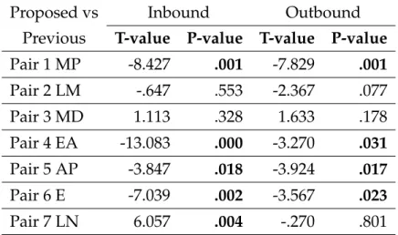
6.4.1 Assessing the Significance . . . 76
6.4.2 Summary . . . 77
7 Assessing the Performance of the Prediction Models 79 7.1 Introduction . . . 79
7.2 Comparison between the Proposed Model and Another Model 79 7.2.1 Experiment Setup. . . 79
7.2.2 Measuring the Performance of Both Models . . . 83
7.2.3 Measuring the Significance . . . 85
7.3 Comparison between the Proposed Model and that in Our Pre- vious Study . . . 87
7.3.1 Experiment Setup. . . 87
7.3.2 Measuring the Performance of Both Models . . . 90
7.4 Summary . . . 93
8 Conclusion and Future Work 95 8.1 Conclusion . . . 95
xii
8.1.1 Results and Findings . . . 95 8.1.2 Research Contribution . . . 97 8.2 Recommendations for Future Research. . . 99
A Publish Work 113
A.1 Journal Paper and Book: . . . 113 A.2 Conference Papers: . . . 113
List of Figures
1.1 Framework of this research . . . 11 3.1 An example of one route where the bus runs between two ad-
jacent bus stops . . . 23 3.2 Interval between two adjacent bus stops . . . 25 3.3 Logarithmic ranges stable and unstable intervals . . . 28 4.1 Daily average of bus travel time over intervals for the inbound
direction . . . 40 4.2 Daily average of bus travel time over intervals for the out-
bound direction . . . 42 4.3 Ratio of stable and unstable Intervals. . . 44 5.1 Observed average travel time over unstable intervals for week-
days . . . 55 5.2 Observed average travel time over unstable intervals for week-
days . . . 57 5.3 Input variables of the model . . . 61 5.4 Training models . . . 62 5.5 Prediction error for the inbound and outbound directions . . . 65 6.1 Establishing the training model . . . 72 6.2 Scheme of the input data . . . 73 6.3 Prediction error for the inbound and the outbound directions 75 7.1 Variable input for the previous model . . . 81
xiv
7.2 Comparison of prediction performance between proposed and HATT-based Models . . . 86 7.3 Training data and prediction iteration . . . 89 7.4 Comparison of prediction performance between proposed and
previous models . . . 91
List of Tables
3.1 Fields of bus probe data . . . 22
3.2 Time Periods . . . 24
3.3 Logarithmic ranges of interval criteria . . . 28
4.1 Periodical variance of travel time over unstable intervals for weekdays . . . 46
4.2 Daily variance of travel time over unstable intervals . . . 47
4.3 Correlation between time periods of a day. In/Out denotes the inbound or the outbound directions . . . 49
5.1 Average MAPE of prediction error . . . 66
5.2 ANOVA t-test of prediction error between SVR, ANN and RF 67 6.1 Comparison for the off-peak periods . . . 74
6.2 Comparison for the peak-hour periods . . . 74
6.3 Paired samples test for the off-peak periods . . . 77
6.4 Paired samples test for the peak-hour periods. . . 77
7.1 Paired sample tests between proposed and HATT-based mod- els . . . 87 7.2 Paired sample test between the proposed and previous models 92
List of Abbreviations
API Application Programming Interface AVI Automatic Vehicle Identification APTIS Automatic Passenger Ticket Issue GPS Global Positioning System
DATT Dynamic Average Travel Time HATT Historical Average Travel Time ITS Intelligent Transportation System
E Early Morning
MP Morning Peak
LM Late Morning
MD MidDay
EA Early Afternoon
AP Afternoon Peak
E Evening
LN Late Night
SVM Support Vector Machine
SVR Support Vector Machine Regression ANN Artificial Neural Network
RF Random Forest
NARX Nonlinear Autoregressive Network with eXogenous Inputs
DT Decision Tree
MSE Mean Square Error
MAPE Mean Absolute Percentage Error RMSE Root Mean Square Error
MLP Multilayer Perceptron
NARMAX Nonlinear Autoregressive Moving Average with eXogenous RBF Radial Basis Function
ARIMA Autoregressive Integrated Moving Average
List of Symbols
Tt Travel Time
tp Time Period
ln Natural Logarithm
d day on weekday
i Interval between Two Bus Stops N Number of Intervals
StDev Standard Deviation
µ Average of Standard Deviations VarStDev Variance of Standard Deviations
σ Standard Deviation of the Standard Deviation
xt Time Series
nsv Number of Support Vector
C Constant
u Random Vector
K Element of Regression Function w Weights of the Network
xi Input Vector yi Scalar Output
Chapter 1
Introduction
This chapter introduces the background of this thesis. It discusses back- ground, problem formulation, the uniqueness of this research, research ob- jectives, and the framework of the research.
1.1 Background
Prediction of travel time on the route is an important factor for many peo- ple who travel or commute, especially using the public bus services. Mostly, passengers consider travel time as well as stochastic factors (variability) such as dwell time, traffic congestion, accidents, and so on. They usually prefer to minimize the time spent traveling from their origin to destination by choos- ing the best route.
On the other hand, travel time variability comes from various sources, which can be divided into two categories: regular variations (recurrent) like e.g. day-to-day variation and irregular condition variations (non-recurrent) like e.g. incidents, weather or random variations [48]. For non-recurrent variations, it is hard to predict the location and time of their occurrence [43]. Therefore, it is hard to predict the bus travel time that would result for passengers from adjusting their departure time in such cases [78], [28].
2 Chapter 1. Introduction By contrast, with known regular and irregular condition-dependent varia- tions, travelers may be able to adjust their departure time or route to arrive on time at their destinations [78].
In recent years, Intelligent Transportation Systems (ITSs) has been widely used in planning, evaluation and control of the reliability of public trans- portation systems [39]. Most public transportation systems such as bus ser- vices have either successfully implemented or are in the process of imple- menting various ITSs applications in their system, with the aim of providing reliable and accurate information for passengers [89], [19], [33].
Over the past several years a number of research projects have attempted to empirically measure behavioral responses to changes in travel time vari- ability [84]. These have generally been built on theoretical models of schedul- ing choice that account for changes in departure time in response to the expected punctuality associated with variability. Using the mean variance model approach, these studies have confirmed that the travel time tends to be influenced by traffic conditions, ridership and weather conditions, which, in turn, may present variability depending on the time periods in the day and the day of the week [32], [27].
On the other hand, an important evolution in Intelligent Transportation Systems (ITSs) is largely due to the availability of bus probe data. Probe data generated by vehicles include data obtainable from navigation systems, such as the time and position (longitude and latitude), i.e. data on the vehicle’s running and performance history [69], [77], [86]. Since these probe data can be obtained continuously over time from a vehicle, they enable monitoring of the state of road traffic characteristics [77]. It is expected that detailed traffic analysis of bus travel times could be carried out using these data before making a prediction model.
1.2 Problem Formulation
In recent years, many studies have been performed to develop models to pre- dict bus travel times on routes, especially arrival times at bus stops. In addi- tion, a number of dynamical models have been proposed to predict bus travel time on roads in urban areas. However, such models are over-simplified and may not represent real conditions because the models do not take into ac- count bus travel time variability on the routes [27], [77].
In summary, previous studies have been conducted in the research field of predicting bus travel/arrival times for a single bus route using the histor- ical average bus travel/arrival time. Furthermore, their prediction models assume that the historical travel time patterns will remain the same even in the future time period in a day . In this case, model precision is highly de- pendent on the amount of the historical traffic pattern data, as the accuracy of analysis results may differ depending on real conditions [30], [63].
In addition, limitations in the volume of historical data make for a sig- nificant difference in the relationship between historical traffic patterns and real conditions. The problem in these methods usually comes from the as- sumption that travel time recurs predictably or the assumption that a regular pattern repeatedly occurs in the same time-period over days [22]. Therefore, the variations in bus travel time on the route are often not sufficiently well- defined to build a prediction model.
Liu et al. [52] noticed that a bus is not operated in the same way as other vehicles. Even though the bus delay is caused by a traffic jam, the bus cannot increase its speed to adjust the delay because the bus speed is limited and they should follow the route that has been determined by a time schedule [52], [16]. Many authors also noticed that delays at the upcoming bus stops depend on accrued variation of travel time at past stops. Bertini et al. [30]
showed that the bus travel time between two adjacent bus stops increases in
4 Chapter 1. Introduction several time periods. Moreover, there are correlations of travel time between time periods, especially two adjacent time periods, which influence the bus travel time in the next time period [55], [77], [71].
In other words, the bus travel time in the previous period will affect the travel time in the next or later period [23]. Likewise, if the trend of the histor- ical travel time is not linear, e.g. when the short-term fluctuations due to acci- dents that happen suddenly in the current period will affect later travel time periods such as the morning peak period, variations in the historical data- set and variations in the relationship between the historical patterns and the current traffic patterns could dramatically affect the prediction in a negative way [78]. Therefore, the performance of these models is highly dependent on the quality of the historical data.
1.3 Uniqueness of this Research
Numerous studies have been conducted to predict the bus travel time be- tween two adjacent bus stops considering the variability of travel time be- tween time periods in a day. However, these models do not give sufficient attention to predicting bus travel time over intervals between adjacent bus stops. The result is that these models do not have the ability to capture the complex non-linear relationship between travel time and variability.
Further, in this thesis, I propose a model for predicting travel time over unstable intervals between adjacent bus stops on the routes during different time periods in a day, since bus travel time over the unstable intervals varies significantly between time periods in a day and in the same time period over days, and there are in addition strong correlations between time periods in a day. In constructing my model, the variability of travel time is the main focus point in the prediction model.
Therefore, I consider using two important independent variables: his- torical average travel time data in the same time period and dynamic av- erage travel time data in the time period just before the current one. Using these independent variables yields a highly accurate performance in dynam- ically predicting bus travel time under recurrent and non-recurrent variabil- ity. Therefore, the model may capture the influence of unexpected events such as accidents, and traffic jams that influence the bus travel time on the routes.
1.4 Research Objective and Scope
The primary objective of this study is to develop a nonlinear dynamical model for predicting bus travel time over unstable intervals between adjacent bus stops in seven and eight time periods in a day. This study uses real bus probe data to develop the model. The study mainly examines the significant fac- tors: variations of travel time between time periods in a day and in the same time periods over days as well as the correlation of travel time between eight time periods in a day, which influences the bus travel time in the current time period. In general, the objectives of this research are outlined as follows:
1. Calculate bus travel time over each interval between two adjacent bus stops in each time period, where I divide a day into eight time periods:
early morning (EM), morning peak (MP), late morning (LM), midday (MD), early afternoon (EA), afternoon Peak (AP), evening (E), and late night (LN). In Section 5, the early morning (EM) period is ignored and only the remaining seven periods are considered.
2. Clarify that the bus travel time shows significant variation depending on the time period and the day.
6 Chapter 1. Introduction 3. Classify intervals between two adjacent bus stops into two classes: sta-
ble and unstable.
4. Establish the variability of bus travel time over unstable intervals be- tween the eight time periods in a day and that in the same time period over days using a statistical test.
5. Provide the correlation of bus travel time over unstable intervals be- tween time periods in a day using a statistical test.
6. Build a model to predict bus travel time over each unstable interval in each of seven and eight time periods in a day. Then, evaluate the prediction model by comparing them with other models.
1.5 Research Framework
Figure 1.1 shows the conceptual framework of this research for predicting bus travel time over each unstable interval. I defined the framework of my study as follows:
1. Data Preparation and Preliminary Analysis: The process begins with the preparation and preliminary analysis of the probe data. I extract the information from bus probe data and observe bus travel time over each interval between two adjacent bus stops in eight time periods in a day over 20 days. This is to show that bus travel times are influenced by each time period, in which traffic conditions, ridership and weather conditions often change even though buses run over the same inter- vals between adjacent bus stops. Then, using the standard deviation of travel time in each time period, I roughly classified all intervals into two classes: stable and unstable. The details are described in Chapters 3and4.
2. Advanced Analysis: This stage covers the variability analysis of travel time over each unstable interval for model development. I conduct three statistical analyses to confirm the variations of the travel time among eight time periods in a day, in the same time periods over days and the correlation of the travel time between adjacent time periods in a day. The details are described in Chapter4.
3. Building of Prediction Models: Considering the results obtained in stage 2, I chose two significant factors influencing the bus travel time over each unstable interval as input parameters of the models. I conducted experiments to predict travel time over unstable intervals focusing on recurrent and non-recurrent variability between the seven time peri- ods in a day. To build the prediction models, I applied a time series approach using three machine learning methods: Artificial Neural Net- work (ANN), Support Vector Machine (SVM) and Random Forest (RF).
The details are described in Chapter5.
4. Establishment of prediction models using another approach which dis- tinguishes off-peak and peak-hour periods: In this stage, I conducted experiments to predict travel time over unstable intervals focusing on off-peak and peak-hour periods for eight time periods in a day. To build the prediction models, I applied the time series approach using two ma- chine learning (ML) techniques: Artificial Neural Network (ANN) and Support Vector Machine (SVM). The details are described in Chapter6.
5. Evaluation and Comparison: I compare the model’s performance using a wide range of different types of data sets to decide which are the most suitable input variables. Then, I identified the influence of different attributes in the input variables which have a significant effect in the prediction results. The details are described in Chapter7.
8 Chapter 1. Introduction
1.6 Research Question
The major research questions of our work concern revealing the factors in- volved in and ways to achieve high-accuracy prediction results from real bus probe data with different parameters of independent variables. There are many parameters that will affect the accuracy of results to be considered be- fore building a prediction model. The following are the research questions addressed in this research.
• Question 1: Are there any differences between travel time over each interval between two adjacent bus stops over the eight time periods in a day?
• Question 2: Is it possible to set boundaries between stable and unstable intervals?
• Question 3: What is the ratio of the unstable intervals to the whole?
• Question 4: Are there any variations in unstable intervals among the eight time periods in a day and among the same time periods over days?
• Question 5: Is there any correlation of travel times over unstable inter- vals among the eight time periods in a day?
• Question 6: Is it possible using nonlinear dynamical models built using machine learning techniques such as ANN, SVM and RF to predict bus travel time over each unstable interval between two adjacent bus stops?
• Question 7: Are there any significant impacts in using different input variables to predict travel time over each unstable interval while distin- guishing between off-peak and peak-hour periods?
1.7 Contributions
Three contributions have been made in this paper. First, the records of bus travel time over each interval between adjacent bus stops were obtained from all of the bus routes during eight time periods in a day over 20 days. Then, the intervals were distinguished into stable and unstable intervals.
Second, I clarified the variability of bus travel times over unstable inter- vals between time periods and in the same time periods over days. I also identified that there are statistically significant correlations of travel time be- tween the eight time periods in a day which influence the bus travel time in the current time period over unstable intervals. Third, I developed nonlin- ear dynamical models to predict bus travel time over each unstable interval between adjacent bus stops. The characteristics of the models are as follows:
1. A prediction model to predict travel time in each of the seven time pe- riods in a day focused on regular variations (recurrent) and irregular condition variations (non-recurrent).
2. A prediction model to predict the bus travel time in each of the eight time periods in a day based on traffic density i.e., off-peak and peak- hour periods. In this model, I demonstrated the impact of two types of input variables for the prediction in off-peak and peak-hour periods.
Finally, to measure the prediction performance, I evaluated the perfor- mance of the models by conducting several experiments. First, I conducted a comparison experiment between our proposed model and the model in other previous study. Second, I compared the proposed model and the model in my previous study.
10 Chapter 1. Introduction
1.8 Thesis Outline
The thesis is organized as follows: Chapter 1 discusses the background, prob- lem formulation, uniqueness, objectives, framework, questions addressed and contribution of this research. Chapter 2 presents a literature review of conceptual, theoretical and methodological topics related to travel time vari- ability and prediction models for bus travel time. Chapter 3 explains the data used in this research, shows how real-world bus probe data can be cal- culated/utilized and introduces briefly several machine learning techniques used. Chapter 4 describes an empirical analysis of the distribution the bus travel times, and shows statistical analyzes to confirm the variations of travel time over each unstable interval. Chapter 5 presents the simulations of the proposed model’s algorithms to predict bus travel time focusing on recur- rent and non-recurrent variabilities of travel time over the unstable intervals.
Chapter 6 provides a different approach for predicting bus travel time con- sidering traffic congestion by distinguishing peak periods from off-peak pe- riods. Chapter 7 presents the model performance evaluation resulting from the comparison experiment between our models and the model proposed by other study , as well as the model in my previous study. In Chapter 8, the thesis concludes with a summary of the results of the experiments and the findings and contributions of this research , and discusses some topics for future scientific research in the prediction of bus travel time.
FIGURE1.1: Framework of this research
Chapter 2
Related Work
2.1 Introduction
This chapter presents a literature review of conceptual, theoretical and method- ological topics related to the prediction of bus travel and arrival time. Through the literature review, the importance of models for the prediction of bus travel/arrival times for passengers and management control of bus travel time became clear. The literature review led to the motivation to test a stochas- tic time series in nonlinear dynamical models for bus travel prediction.
2.2 Travel Time Variability
Travel time variability reflects the degree of variation in the travel time of a trip that is recurrent or non-recurrent over several time periods in a day or day to day [73]. Traffic congestion as a source of travel time variability should be analyzed by distinguishing recurrent congestion (e.g., the daily increase in traffic during the peak hour periods on weekdays) and non-recurrent conges- tion, which is caused by infrequent incidents such as accidents and extreme weather [22], [43].
Travel time variability is a key factor that passengers consider when mak- ing basic travel decisions regarding destination, route and departure time,
14 Chapter 2. Related Work and numerous studies have attempted to measure travel time variability us- ing two modeling approaches: the scheduling model and the mean variance model [3], [9], [12], [43]. Measuring travel time variability enables greater support for the prediciton of travel time either with empirical, analytic or simulation methods [9]. Over the last several years many studies have in- vestigated bus travel time variability on routes in urban networks, especially between adjacent bus stops along the route. Using the mean variance model approach, these studies confirmed that travel time tends to be influenced by traffic conditions, ridership and weather conditions, which, in turn, may vary depending on time period in a day and the day of the week [3], [9], [78].
Uno et al. [77] proposed a methodology for evaluating the road network from the viewpoint of travel time stability and reliability using bus probe data. Travel time distributions of arbitrary routes are estimated by statisti- cally and directly summing up observed multiple travel time distributions.
In their study, probe data can be applied to the tasks of automatic incident detection and observations of travel time and its variability.
In addtion, Gurmu [35] and E Durán-Hormazábal [43] conducted an anal- ysis of bus travel time variability before building a prediction model. The model demonstrated its superior performance in terms of mean absolute per- centage error (MAPE). Patnaik et al. [63] carried out an analysis of travel time variability over the eight time periods in a day. Their model could also pre- dict bus arrival times for various conditions.
2.3 Methodology of Travel Time Prediction
A variety of models and algorithms have been developed to predict bus ar- rival times or bus travel times. The most widely used models can be classified into the following categories: historical average models, regression/time se- ries models, Machine Learning Techniques (ML) including Artificial Neural
Network (ANN), Support Vector Regression(SVR) and Random Forest (RF).
2.3.1 Historical Average Model with Time Series Approach
Over the last several years, many researchers have empirically attempted to predict travel time over a route using historical average travel time directly or without combination with other inputs [7], [74], [71]. Historical average models are based on the historical data and able to predict the bus travel time or bus arrival time from previous bus trips. These models will be practical, useful, and reliable. Gurmu and Nall [9] developed a historical data model for predicting the link travel time between two bus stops, which was calcu- lated as the average travel time between two bus stops minus the average dwell time at the bus stops. Patnaik et al. [43] also suggested a historical approach in their study and showed good results.
The strength of historical time series data models is high computation speed due to the simple formulation of the algorithm. The models do not need a large number of travel time variables, but only time-related data [85], [44], [92]. The models could be built only from historical data, without dy- namic observations [18]. However, the main disadvantage of this type of model is the averaging of input data over time. The predictions of travel time tend to concentrate on the trend of the historical travel time data and become problematic if the trend is not linear, e.g. if short-term fluctuations due to an accident that happened suddenly in the early morning affect later travel time such as in the morning peak [28], [50]. Variations in the historical data- set and variations in the relationship between the historical patterns and the current traffic patterns could dramatically affect the prediction in a negative way [41]. Moreover, the performance of these models is highly dependent on the quality of the historical time series dataset, which is not always available [19], [92], [62].
16 Chapter 2. Related Work Furthermore, a lot of proposed studies also discuss historical average travel time using regression models. In addition, their models require a linear mathematical function to explain a dependent variable with a set of indepen- dent variables [90]. Unlike the previous models, these are able to work satis- factorily even if traffic conditions are not stable. They usually measure the si- multaneous impact of various factors, which are independent of one another, affecting the dependent variable. For example, Patnaik et al. [63] developed a set of multiple linear regression models to estimate bus arrival times using distance, number of stops, dwell times, number of boarding and alighting passengers and weather descriptors as independent variables. Their study showed that the models could be used to estimate bus arrival/travel time at downstream stops.
Jeong and Rilett [40] and Ramakrishna et al. [65] also developed mul- tiple linear regression models using different sets of independent variables.
In their studies, the regression models outperformed the time series model.
However, these models have a relative advantage in revealing which inde- pendent variables are less or more important for predicting travel times. For example, Patnaik et al. [63] mentioned that weather was not an important input in their model. Ramakrishna et al. [65] also found that two variables, i.e. bus stop dwell times from the origin of the route to the current bus stop in minutes and intersection delays from the origin of the route to the current bus stop in minutes, are less important in predicting bus travel time. Be- cause variables in bus travel time are inter-correlated between time periods, the applicability of the regression models is in general limited [21], [74], [16].
On the other hand, machine learning techniques have recently gained popularity in predicting bus arrival/travel time. These techniques have also been used in several large-scale prediction competitions and suggest that by combining the model with the time series approach, the prediction accuracy can often be improved [47], [9].
2.3.2 Machine Learning Techniques
Machine learning (ML), which is a branch of artificial intelligence, is about the construction and study of systems that can learn from data. ML methods consist of two stages, i.e., choosing a candidate model, and next, predicting the parameters of the model through a learning process based on existing data [29]. ML methods have certain benefits with respect to statistical meth- ods in the following respects: dealing with complex relationships between predictors that can come up within a huge volume of information, process- ing non-linear relationships between predictors, and processing complicated and noisy data. These models can be used for prediction of travel time, with- out implicitly addressing the traffic data [47], [9], [29]. Results obtained for one location are normally not transferable to the next, because of location- specific circumstances, e.g., geometry or traffic control.
In recent years, machine learning techniques (ML) have commonly been used to predict travel time because of their ability to solve complex non- linear relationships. ANN was demonstrated as a potential method for pre- dicting travel time. Chung, E. H., and Shalaby, A. [71], Bai et al. [9], Gurmu et al. [35], [29] developed models to predict bus arrival time with a variety of traffic conditions and introduced an ANN model based on historical data such as Automatic Vehicle Location (AVL), Automatic Passenger Ticket Issue System (APTIS) and GPS data. Their proposed models are suitable for find- ing complex nonlinear relationships between the dependent variable of bus travel time and the independent variables that influence the travel time [11], [42]. Moreover, these are data-driven techniques and require a large set of data for better learning. Also, they are problem-specific models and when- ever the input variables change, the whole model has to be restructured [83].
On the other hand, a lot of studies [2], [9], [19], [34], [85], have employed other machine learning techniques such as Support Vector Machine (SVM)
18 Chapter 2. Related Work and Random Forest (RF) to build prediction models for bus travel time and showed that these models were practical, useful and reliable, where the traf- fic flow was relatively small and stable.
In addition, RF has also been applied to prediction of bus travel time un- der traffic flows and showed that the model outperformed other models in terms of prediction precision [34], [58] [36], [46]. Although their work uses bus historical data with a consideration of traffic conditions and with theday divided into several time periods, their model only focuses on a number of routes in certain corridors.
In order to construct a prediction model using real travel time data (his- torical), previous studies employed a combination of ML and time series model. Next, their model explicitly incorporated information about season- ality into the data (time period of a day and day of a week, etc) using bus probe data [5], [29], [35], [80]. The models confirmed that the developed model could be applied to predict short-term travel time with various condi- tions. However, they have not discussed a model for predicting travel time over each unstable interval between adjacent bus stops considering the vari- ability of travel time over time periods and days.
Moreover, the literature survey shows that most reported studies about bus travel time/arrival time prediction have been developed for homoge- neous traffic conditions only. This is because heterogeneous traffic conditions are very complex and even their analysis to build a prediction model may be more challenging [8], [61], [64].
2.4 Summary
The above literature review of the models and algorithms for bus travel time prediction shows that many models are based on historical patterns and other variables correlated with the arrival/travel time. The variables used
include real data about historical arrival or travel time, dwell time, number of stops along the route, distance between adjacent stops and the road char- acteristics. They are from data collections such as, AVL, APTIS, survey and Probe data.
History-based models assume that the conditions of traffic do not change much, which may not be true when considering a switch from off-peak to peak-hour and vice versa. These models were mainly used in areas where congestion is minimal because they assumed traffic conditions are similar (homogeneous). However, it could be argued that it is also possible to ob- serve such patterns in areas where the congestion is severe. This can be found out from extensive historical data analysis by looking into the distribution of travel time between time periods over days or days of the week and so on.
In areas where stable demand and similar traffic patterns exist, history-based models are able to give satisfactory bus travel time information. So there is no need to go for complex prediction models. Machine learning techniques such as ANN, SVR and RF have outperformed other methods in cases where enough data is available.
However, to greatly improve the prediction accuracy of travel time, we should first focus on shorter intervals on a route, such as the intervals be- tween adjacent bus stops, considering the variability of travel time between them. Furthermore, it is difficult in practice to determine whether or not a time series of travel time recurs and whether a regular pattern repeatedly occurring in the same time period over days becomes a homogeneous or het- erogeneous traffic pattern. This heterogeneity, coupled with variability of travel time on the road makes bus travel time prediction more challenging than can be handled by the reported proposed model. There is, therefore, a need for models that can capture the stochastic behavior of traffic character- istics with a large data requirement.
The present study will be an attempt in this direction to develop nonlinear
20 Chapter 2. Related Work dynamical models for predicting bus travel time. For this purpose, at first, I classified intervals between two adjacent bus stops into two classes: stable and unstable. Next, I identified two statistically significant factors: varia- tions of travel time in the same time periods over days and the correlation of travel time between the seven or eight time periods, which influences the bus travel time in the current time period over unstable intervals. Then, I developed nonlinear dynamical models for predicting bus travel time over each unstable interval between adjacent bus stops in each of seven or eight time periods in a day.
Chapter 3
Data and Methodologies
3.1 Introduction
This chapter explains the data used in this research, describes the preliminary data preparation for calculation and the methods of prediction models. The present study shows how real-world bus probe data can be utilized, how the data should be calculated, how to distinguish stable intervals from unstable intervals and introduces briefly several machine learning techniques used.
3.2 Probe Data
3.2.1 Overview
Probe data generated by vehicles includes data obtainable from navigation systems, such as the time and position (longitude and latitude), i.e. data on the vehicle’s running history, and front-rear acceleration or right-left acceler- ation, i.e. data on the vehicle’s performance history. Since these probe data can be obtained continuously over time from the vehicle, they allow moni- toring of the state of road traffic at any chosen location or point in time and the detection of traction information. Thus probe data offers the potential to develop a prediction model that can improve the accuracy of prediction results [6], [69], [77].
22 Chapter 3. Data and Methodologies A typical unit of travel time for a bus on a route is the time required to move from one bus stop to the next, as shown in Figure3.1, when a bus ar- rives at and departs from adjacent bus stops along route. A bus will travel on the same segment twice in a single trip [70], [45], but in the opposite direction i.e, the inbound and outbound directions.
3.2.2 Bus Probe Data
The probe data used in this research were provided by NISHITETSU Bus Company. The data were collected from the 21st of November to the 20th of December 2013. The probe data include GPS information on bus po- sitions, time information indicating when the GPS information was taken, route number, number of bus stops, travel direction and so on. Bus routes are operated for around 18 hours a day. Buses run in different patterns on weekdays, Saturdays and Sundays/holidays according to their time tables.
TABLE3.1: Fields of bus probe data
Field Description
Vehicle Id Bus identity number
Lat & long GPS Position of Latitude and Longitude Direction Inbound or outbound
GPS time Time obtained by GPS
Route Number The number assigned to a route Type of Route Sub route number
Bus number The order of a bus running on a route Bus stop code A code number assigned to a bus stop
Bus pole code A code number assigned to a pole of a bus stop Here, in this study, I have just dealt with travel time on weekdays, not Saturdays or Sundays/holidays because of the lack of data volume. I ana- lyzed 175 routes consisting of 6129 intervals for the inbound direction and 5700 intervals for the outbound direction, on which 2045 buses a day were operated. Travel time information is recorded every 3 minutes and at the
FIGURE3.1:Anexampleofoneroutewherethebusrunsbetweentwoadjacentbusstops
24 Chapter 3. Data and Methodologies time when a bus stops. Table3.1shows a summary of bus probe data used in this study. In addition, the bus trips are classified in the database into eight different time periods, as shown in Table3.2.
3.3 Methodologies
3.3.1 Travel Time over Intervals
In order to calculate bus travel time, first I calculated the average travel times over each interval during each of the eight time periods in a day. This is because bus travel times are influenced by each time period, in which traffic conditions, ridership and weather conditions often change even though the buses run over the same intervals between adjacent bus stops [3], [35], [63], [86].
Then, I calculated the average travel time over each interval in each time period in a day for 20 days, because the travel time may usually vary dur- ing the day. For short, I will just use the term "interval" below, when I mean
"travel time over interval between adjacent bus stops", where the classifica- tion and definition of the time periods are shown in Table3.2and a bus travel time interval is illustrated in Figure3.2.
TABLE3.2: Time Periods
Periods Ranges of Time Early Morning (EM) 5:00:00-7:29:59 Morning Peak (MP) 7:30:00-9:29:59 Late Morning (LM) 9:30:00-11:59:59 Midday (MD) 12:00:00-12:59:59 Early Afternoon (EA) 13:00:00-15:29:59 Afternoon Peak (AP) 15:30:00-17:29:59 Evening (E) 17:30:00-19:29:59 Late Night (LN) 19:30:00-25:59:59.
FIGURE3.2: Interval between two adjacent bus stops
The following shows how to calculate bus travel time over an interval between adjacent bus stops. I define travel time TtAB(i,tp,d), which is the length of time when bus #iruns between adjacent bus stops: AandB, in time periodtp(∈ (EM, MP, LM, MD, EA, AP, E, LN)) on a dayd, which is always a weekday in this paper,
as follows:
TtAB(i,tp,d) =tB(i,tp,d)−tA(i,tp,d), (3.1) where tB(i,tp,d) and tA(i,tp,d) are the time when the bus #iarrives at bus stopBand departs from bus stop Ain time period (tp) on a day (d), respec- tively. Using equation (3.2), we calculate the average travel time Tt(tp) in each of 8 time periods (tp) in a day as follows:
TtAB(tp,d) = 1 N
∑
N i=1TtAB(i,tp,d), (3.2)
where N is the number of buses running on the interval between adjacent bus stops A and B, and may vary according to each interval in the specific time period. In what follows, we refer to each average travel time between adjacent bus stops for each of the eight time periods in day as an interval.
26 Chapter 3. Data and Methodologies
3.3.2 Distinguishing Stable and Unstable Intervals
The variability of bus travel time can be categorized by its time frame. Maria et al. [54] discussed variability as occuring between time periods in a day or between days. The variability is caused by unexpected events such as construction or inclement weather or generally refers to changes in travel time due to peak-hour congestion.
In addition to periodical and daily variations in travel time, it may be of interest to compare the average travel time between time periods in a day.
Other studies suggest that travel times may vary for different time periods in a day due to changes in vehicle volume, construction etc. However, in the same time periods travel times should be similar for various days of the week in the absence of unexpected events. In this work, average travel time data for each of the eight time periods in a day are compared.
First, using equation (3.3), I calculate the average travel timeTti(tp)over intervalsiin time periodtpovernweekdays, wheren=20.
Tti(tp) = 1 n
∑
n d=1Tti(tp,d) (3.3)
Then, I put a number onto each interval from 1 toN, where Nis the total number of intervals; I calculate Tti, which is the average travel time over intervalsi (1 ≤ i ≤ N) among TP = {EM,MP,LM,MD,EA,AP,E,LN}, a set of eight time periods of a day using equation (3.4).
Tti = 1
|TP|
∑
tp∈TP
Tti(tp) (3.4)
To transform all the data to normal distribution, I transform the data of the average travel time over intervals (Tti) among time periods (TP) in a day using natural logarithm.
Next, I calculate StDevi, which is the standard deviation of the average
travel time over intervalsito find out whether travel time over each interval is stable or not. To make a fair comparison for all routes considering the differences of distance of all the intervals, I divide the standard deviation of the average travel time over each interval by the average travel time over the interval using equation (3.5).
StDevi = q 1
|TP|∑tp∈TP(Tti(tp)−Tti)2
Tti (3.5)
The second step is to create logarithmic ranges to distinguish criteria for stable and unstable intervals of travel time over each interval as shown in Figure3.3. I calculate σ, the standard deviation of the standard deviation of the average travel time over all the intervals using equation (3.6).
σ= s
∑Ni=1(StDevi−µ)2
N−1 (3.6)
Hereµin equation (3.7) is the average of the standard deviation over the intervals.
µ = 1 N
∑
N i=1(StDevi) (3.7)
Next, I calculate the standard deviations of the average travel time over interval i (1 ≤ i ≤ N,whereN is number of intervals) for each of the eight time periods in a day using equation (3.8)
StDev(Tti) = q
Var(Tti) (3.8)
28 Chapter 3. Data and Methodologies
FIGURE3.3: Logarithmic ranges stable and unstable intervals
According to StDevi, interval i is classified into logarithm ranges of in- terval criteria as shown in Figure3.3 and Table 3.3. I roughly classified all intervals into two classes: stable and unstable; if the standard deviation of travel time over an interval is less than µ, then the interval is classified as stable, or otherwise, unstable. Then, I further classified each of the two into three sub-classes: weak, medium and strong (we present the results in Sec- tion4.4). The criteria for each subcategory are as follows:
TABLE3.3: Logarithmic ranges of interval criteria Interval Category Logarithmic Ranges Strong stable ifStDevi<=µ−2σ
Medium Stable ifµ−2σ <StDevi <=µ−σ Weak Stable ifµ−σ <StDevi <=µ−σ Weak Unstable ifµ <StDevi <µ+σ
Medium Unstable ifµ+σ <=StDevi <µ+2σ Strong Unstable ifStDevi>=µ+2σ
3.4 Methods of Travel Time Prediction
In this Section, I briefly present references and an outline for nonlinear time series prediction using the machine learning techniques Artificial Neural Net- work with NARX, Support Vector Regression (SVR) and Random Forest (RF) Regression.
3.4.1 Time Series Approach
The purpose of this section is to provide a brief sketch of time series predic- tion theory. The accuracy of time series prediction is fundamental to many decision processes and hence research to improve the effectiveness of predic- tion models has been ongoing. Successful time series prediction is a major goal in many areas of travel time prediction. However, the time series data are often full of non-linearity and irregularity. There are vast amounts of tech- nical references, books, and journal articles detailing time series prediction algorithms and theory for both linear and non-linear prediction applications [13], [68].
Fundamentally, "the goal of time series prediction is to estimate some fu- ture value based on current and past data samples" [68]. Mathematically, the prediction approach is stated as follows:
ˆ
x(t+∆t) = f(x(t−a),x(t−b),x(t−c)), (3.9) where, in this specific example, ˆxis the predicted value of a (one dimen- sional) discrete time seriesx. "The objective of time series prediction is to find a function f(x)such that ˆx, the predicted value of the time series at a future point in time isunbiasedandconsistent. Whereiis an index to a discrete time series value and N is the total number of samples. It should be noted that an- other measure of a predictor’s goodness is efficiency as related to bias. If the
30 Chapter 3. Data and Methodologies estimator achieves this bound, then it is said to be efficient" [38]. Estimators generally fall into two categories: linear and nonlinear. Over the past several decades, a vast amount of technical literature has been written about linear prediction: "the estimation of a future value based on the linear combination of past and present values" [68]. Real-world time series prediction applica- tions generally do not fall into the category of linear prediction. Instead, they are typically characterized by non-linear models. Therefore, most non-linear models can be handled by machine learning techniques such as, ANN, SVM and RF [13], [68].
3.4.2 Artificial Neural Network (ANN)
I use an ANN-based time series prediction method to predict travel time over intervals between adjacent bus stops on all of the routes. The method is based on a Nonlinear Auto Regressive model with the eXogenous input (NARX) model. The NARX model is well-suited for modeling dynamic non- linear systems, especially those with time series characteristics. In addition,
"NARX model is a subset of the Nonlinear Auto-Regressive Moving Aver- age with Exogenous Inputs (NARMAX), which are nonlinear non-parametric identification models" [26], [87].
The mathematical function which models a real-world system is very complex and usually unknown. However, the NARX model can be con- structed using a simpler function structure such as neural networks [20]. The NARX model formulation [20], [26] is described as follows:
y(t) = f(y(t−1), ...,y(t−ny),u(t−1), ...,u(t−nu)) +e(t) (3.10)
, wherey(t), u(t) and e(t) are the model output, model input, and noise at time t, respectively. ny and nu are the maximum lags in the output and the input, respectively; f(.)is some vector-valued non-linear function, but can be
approximated using some known simpler function such as neural networks [20].
In my model, I used a multilayer perceptron (MLP) with a single hidden layer to approximate any bounded continuous function. The MLP contains one or more layers of hidden units. "The hidden units enable the MLP to learn complex tasks and meaningful features from the input/output relation- ships" [57]. Moreover, "high degree of connectivity between the MLP layers is determined by the weights of the network" [87]. I conducted MLP train- ing with the Levenberg-Marquardt algorithm and evaluated the model using the measure of mean squared error (MSE) in training and testing. The MSE is a default indicator in training the ANN model. The ANN model with the smallest MSE value is considered to be the best model.
3.4.3 Support Vector Machine Regression (SVR)
"Support Vector Machine (SVM) has been developed to work on a non-linear problem by incorporating the concept of the kernel in high-dimensional space;
SVR is an application of SVM to the case of regression" [81], which was de- signed to overcome the over-fitting and to yield a good performance [79], [85].
I assume there arennumbers of training data(xi,yi)(i=1, . . . ,n), where xi is an input vector, and yi is a scalar output. With SVR, I want to assign a function f(x), which has the significant deviation εfrom the actual target yi for all training data. If the value of εbecomes equal or near to 0, a good regression model is obtained [85].
The main purpose of the SVR model is to construct a linear model inm- dimensional feature space which inputxis mapped onto. Using mathemati- cal notation, the linear model f(x,w)is given below [59], [10]
32 Chapter 3. Data and Methodologies
f(x,w) =
∑
n j=1wjgj(x) +b (3.11) , where wj and gj(x) denote the jth weight and nonlinear transformation, respectively, and b is a bias. Next, prediction performance is measured by the loss function L(y, f(x,w)). SVR uses a new type of loss function called ε-insensitive loss function proposed by Vapnik [81]:
Lε(y, f(x,w)) =
0 i f|y− f(x,w)| ≤ε
|y− f(x,w)| −ε otherwise
(3.12)
"SVR performs linear regression in the high-dimensional feature space us- ingε-insensitive loss, and at the same time, tries to reduce model complexity by minimizing ||w||2. This can be described by introducing (non-negative) slack variablesζi,ζ∗i(i =1, . . . ,n), to measure the deviation of training data outside theε-insensitive zone" [59]. Thus SVR is formulated as a minimiza- tion of the following function:
R(w,ζ) = 1
2||w||2+C
∑
n i=1(ζi+ζ∗i) (3.13)
subject to :
yi− f(xi,w)≤ε+ζi∗ f(xi,w)−yi ≤ε+ζi
ζi,ζ∗i ≥0,(i =1, ...,n)
(3.14)
, where(1/2)||w||2is a weight vector norm, and C is a regularized con- stant determining the trade-off between the empirical error and the regular- ized term. εis called the tube size of SVR and it is equivalent to the approx- imation accuracy placed on the training data points [10]. By introducing op- timal constraints, this optimization problem can be transformed into a dual
problem whose solution is given by:
f(x) =
nsv i
∑
=1(ai−a∗i).K(xi,x) +b (3.15) subject to : 0≤a∗i ≤C, 0≤ai ≤C
, wherensv is the number of Support Vector (SVs) andKis a kernel func- tion. "The kernel parameters should be carefully chosen as they implicitly define the structure of high dimensional features and thus controls the com- plexity of the final solution. However, generalization performance, here pre- diction accuracy, depends on a good setting for parameters C, ε, kernel pa- rameters, and input values(x)of the training data" [59].
I selected Radial Basis Function (RBF) as the kernel function in this study.
For measurement of performance (C) in the training process, I selected RBF network (λ,ε) at the minimum error as an SVR model [59].
3.4.4 Random Forest (RF)
The present Section is not intended to provide a detailed description of Ran- dom Forest (RF); the parameters are described in Section5.3.
"Random Forest (RF) Regression is a regression technique that combines the performance of numerous Decision Tree (DT) algorithms to predict the value of a variable" [14]. Therefore, regression using RF can be implemented for time series prediction purposes. That is, when RF receives auinput vec- tor, made up of the values of the different evidential feature analyses for a given training area, RF buildsknumbers of regression trees and averages the results [91], [24], [51].
"Assumed that the u is a random vector with k elements, the aim is to predictvby estimating the regression function:
m(u) = E[v|u =u] (3.16)
34 Chapter 3. Data and Methodologies given fitting sample:
Ss = ((u1v1), ...,(us,vs)) (3.17) which are independent realizations of the random variable(uv). Therefore, the aim is to construct an estimatems of the functionm.
A random forest is a predictor constructed by growing M randomized regression trees. For the j-th tree in the family, the predicted value at u is denoted byms(u;θj,Ss), whereθ1, ...,θMare independent random variables, distributed as θ and independent of Ss. The random variable θ is used to resample the fitting set prior to the growing of individual trees and to se- lect the successive directions for splitting" [76]. The prediction is then given by the average of the predicted values of all trees. Before constructing each tree, the observations are randomly chosen from the elements of u. These observations are used for growing the tree.
"To avoid the correlation of the different trees, RF increases the diversity of the trees by making them grow from different training data subsets created through a procedure called bagging. Hence, some data may be used more than once in the training, while other data might never be used. Thus, greater stability is achieved, as it makes it more robust when facing slight variations in input data and, at the same time, it increases prediction accuracy" [14], [82].
On the other hand, when RF makes a tree grow, it uses the best feature or split point within a subset of evidential features which has been selected randomly from the overall set of input evidential features. "Therefore, this can decrease the strength of every single tree, but it reduces the correlation between the trees, which reduces the generalization error" [14].
"Another characteristic of interest is that the trees of an RF classifier grow with no pruning, which makes them light, from a computational perspective"
[67]. However, "The performance of the RF algorithm depends on the tuning