量子スピン系における磁化率の異常に関する研究

(1)

九州大学学術情報リポジトリ

Kyushu University Institutional Repository

量子スピン系における磁化率の異常に関する研究

相場, 信孝

http://hdl.handle.net/2324/4474935

出版情報：Kyushu University, 2020, 博士（理学）, 課程博士バージョン：

権利関係：

(2)

Doctoral Thesis

On the anomaly of susceptibility for quantum spin systems

Nobutaka Aiba

Department of Physics, Kyushu University, Fukuoka,

819-0395, Japan

(3)

Abstract

In this thesis, we propose a novel method of evaluating an anomaly by investigat- ing the magnetic susceptibility χ and the fourth derivativeA of the energy with respect to magnetization. The term ‘anomaly’ means a divergence in the thermodynamic limit. This anomaly usually marks a phase transition. Researchers have studied the anomaly of the magnetic susceptibility from exact solutions. However, few investigations of high-order differentials such asAhave been carried out. We show that the method observing the anomaly by χ and A is appropriate for the analysis of the phase transition, compared with the method using the magnetic susceptibility χ alone. The introduction of A resolves the issue of whether the high-order differential of energy diverges.

As an example, we apply this method to theS = 1/2XXZ antiferromagnetic chain, which shows a ferromagnetic phase for ∆ ≤ −1, Tomonaga–Luttinger (TL) phase for −1 < ∆ ≤ 1, and antiferromagnetic phase for∆ > 1. ∆ is an anisotropic parameter with thez component of the XXZ antiferromagnetic chain.

The lowest energy of the chain is calculated by numerical diagonalization. Sub- sequently, we analyze the anomalies ofχandAto observe the phase transition.

The results demonstrate that an anomaly ofχ⁻¹ at zero magnetization exists under ∆ > 1, while A at zero magnetization shows an anomaly for ∆ > 1/2.

Hence, the anomaly of A is easier to observe than that of χ. We then consider the anomaly from the perspective of the scaling dimension which indicates the critical phenomena. The scaling dimension of the chain is subject to the parameter

∆. For ∆ = 1, the scaling dimension changes from irrelevant to relevant for U(1)symmetry. This change of the scaling dimension means the phase transition corresponding to the Kosterlitz–Thouless (KT) transition. In contrast, for −1 <

∆≤1region that shows Tomonaga–Luttinger (TL) phase, the scaling dimension is irrelevant. For∆ = 2region that shows the antiferromagnetic phase, the scaling dimensionx_T is relevant in∆ > 1. Thus, we conclude that the anomaly ofAat 1/2<∆<1is different from that ofAat∆ = 1and does not indicate the phase transition. Moreover, we reveal that TL phase is divided into two phases with a

∆ = 1/2boundary by the behavior ofA. We refer to−1<∆<1/2as TL phase (I) and1/2<∆≤1as TL phase (II).

(4)

These ﬁndings indicate that the method usingAis better than that usingχfor analyzing critical phenomena with phase transitions.

(5)

Chapter 1 Introduction

1.1 Condensed matter and spin

In condensed matter physics, phase transitions and their corresponding energy gaps are important research subjects. Researching these gaps is necessary for studying the behavior of quantum spin systems. Bethe showed that an S = 1/2 antiferromagnetic Heisenberg chain had the characteristic of the absence of a gap [1]. In addition, it was conﬁrmed that the correlation function for the system decreases with a power low. Later, Haldane argued the difference between half-odd-integer and integer spin antiferromagnet chains [2]. For the integer spin case, Haldane showed that the antiferromagnetic Heisenberg chain have a gap and the correlation function is exponentially decreased.

Many researchers have observed the energy gap via the magnetization curve as a function of the magnetic field. The magnetic field at zero magnetization is equal to the magnitude of the gap. However, the method of observing the gap via the magnetization curve is not appropriate for deciding whether a spin system is gapless or gapped in numerical calculation; it is difficult to distinguish a gapless system from one with a very small energy gap [3]. Hence, Sakai and Nakano [4, 5, 6, 7] proposed a method for distinguishing a gapless system from a gapped system. In the next section, we introduce Sakai and Nakano’s method.

1.2 Anomaly of magnetic susceptibility

In this section, we review Sakai and Nakano’s work [4], which shows a method for distinguishing a gapless from a gapped system and an anomaly of magnetic susceptibility. The term ‘anomaly’ means that the magnetic susceptibility diverges in the thermodynamic limit.

(8)

First, they focus on the spinS = 1/2square lattice antiferromagnetic Heisen- berg model in two dimensional systems. The Hamiltonian of the model is given by

Hˆ =J₁X

⟨i,j⟩

( ˆS_i^xSˆ_j^x+ ˆS_i^ySˆ_j^y+ ˆS_i^zSˆ_j^z) +J₂X

⟨k,l⟩

( ˆS_k^xSˆ_l^x+ ˆS_k^ySˆ_l^y+ ˆS_k^zSˆ_l^z), (1.1) whereJ₁, J₂ are an exchange interaction,Sˆ_i,Sˆ_j,Sˆ_k,Sˆ_l are the spin operator, and

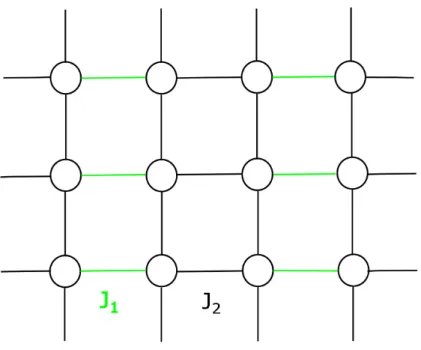
⟨i, j⟩and⟨k, l⟩indicate the nearest neighbor pairs on the lattice. Figure1.1shows the model (1.1). In J₁ ≫ J₂, neighboring spins form pair, which indicates a spin-singlet state (Fig.1.2). Subsequently, the lowest energyE(N, M)and mag- netizationM of the model (1.1) are deﬁned as

Hˆ|ϕ⟩=E(N, M)|ϕ⟩, XN

j=1

Sˆ_j^z|ϕ⟩=M|ϕ⟩,

whereN is the system size,M is a magnetization,Sˆ_j^zis thejth spin operator inz direction, and|ϕ⟩is the eigenstate. We note that|ϕ⟩is a simultaneous eigenstate of Hˆ and P

jSˆ_j^z. To calculate the lowest energy, a numerical diagonalization method is used under a periodic boundary condition. The interaction to the exter- nal magnetic ﬁeldhis

Hˆz =−h XN

j=1

Sˆ_j^z. (1.2)

In the thermodynamic limit (N → ∞), the lowest energy ofHˆper site,ϵ(m), is deﬁned as

Nlim→∞

E(N, M)

N =ϵ(m), (1.3)

wherem = M/M_sis a magnetization normalized andM_s = SN is a saturation magnetization which means the magnetization of the state where all the spins are aligned in the z direction. They then consider ϵ^′′(m)and ϵ^′(m). When ϵ(m)is analytic, the spin excitation energyE(N, M+ 1)−E(N, M)becomes

1

N(E(N, M + 1)−E(N, M))≃ϵ

m+ 1 N S

−ϵ(m). (1.4) From Taylor expansion ofϵ m+_{N S}¹

, Eq. (1.4) is written as E(N, M + 1)−E(N, M)≃ 1

Sϵ^′(m) + 1

2N S²ϵ^′′(m) +· · ·. (1.5)

(9)

Similarly, the spin excitation energyE(N, M)−E(N, M−1)becomes E(N, M)−E(N, M −1)≃ 1

Sϵ^′(m)− 1

2N S²ϵ^′′(m) +· · ·. (1.6) From Eq. (1.5) and Eq. (1.6),ϵ^′′(m)is given by

(E(N, M + 1)−E(N, M))−(E(N, M)−E(N, M −1))≃ 1

N S²ϵ^′′(m).

(1.7) This indicates that ϵ^′′(m)is represented by the difference of energies. By mini- mizing the energy of total Hamiltonian including Eq. (1.1) and Eq. (1.2),ϵ^′(m)is written as

∂

∂m

E(N, M)

N −hM N

= 0 h= ϵ^′(m)

S . (1.8)

Asϵ(m)is assumed to be analytic,ϵ^′(0)becomes zero. Conversely, assuming that ϵ(m)is not analytic,ϵ^′(0)becomes ﬁnite.

The derivative ofmwith respect tohis deﬁned as χ≡ dm

dh = S

ϵ^′′(m), (1.9)

whereχis a magnetic susceptibility. In particular, in the case ofm = 0, Eq. (1.7) is written as follows

2∆_{N S} ≃ 1

N S²ϵ^′′(0), (1.10)

where∆_{N S} =E(N,1)−E(N,0)is the spin energy gap. Whenχ(m = 0) = 0, ϵ^′′(m = 0)is inﬁnite in the thermodynamic limit. In contrast, whenχ(m= 0)̸= 0, ϵ^′′(m = 0) = 0in the thermodynamic limit. In the thermodynamic limit, the relation betweenχand∆_{N S} is











Nlim→∞χ(m= 0) = 0

⇒∆_{N S} =ﬁnite (gapped),

Nlim→∞χ(m= 0)̸= 0

⇒∆_{N S} = 0 (gapless).

(1.11) (1.12)

This indicates whether the spin systems is gapless or gapped from the numerical results ofχ.

(10)

The model (1.1) is gapless forα > α_cwhereα_c= 0.52337(3)andα =J₁/J₂, while this model is gapped forα < α_c [8]. They then calculate χfor the model (1.1). Figure1.3 shows the magnetization dependence ofχ for the model (1.1).

Figure1.3(a)shows that the curve is smooth andχ̸= 0atm= 0forα=J₂/J₁ = 1. Conversely, Fig.1.3(b)shows thatχ = 0 atm = 0forα =J₂/J₁ = 0.2, and χseems to diverge nearm = 0in the thermodynamic limit. The divergence near m = 0in Fig. 1.3(b) means the anomaly of magnetic susceptibility. Figure 1.4 shows the1/N dependence ofχatm = 0. Figure1.4(a)indicates thatχatm = 0 becomes ﬁnite in the thermodynamic limit. In contrast, Fig.1.4(b)indicates that χatm = 0becomes zero in the thermodynamic limit. Thus, the numerical results of χ demonstrate that the model (1.1) is gapless for α = 1 and is gapped for α = 0.2.

These results indicate that they propose a method for distinguishing a gapless system from a gapped system by using magnetic susceptibilityχ. We focus on the anomaly of magnetic susceptibilityχnear zero magnetization in Fig.1.3(b). The term ‘anomaly’ refers to a divergence in the thermodynamic limit. This anomaly usually exhibits a phase transition.

Fig. 1.1:Square lattice antiferromagnetic Heisenberg model. The solid green line and black line are the exchange interactionJ₁and the exchange interactionJ₂of the model (1.1).

(11)

Fig. 1.2:Spin-singlet state that neighboring spins form pair when the exchange interac- tionsJ1 ≫J2of the model (1.1).

(a) gapless (b) gapped

Fig. 1.3:Magnetization M/M_s = m dependence of the magnetic susceptibility χ for S = 1/2square lattice antiferromagnetic Heisenberg model (1.1) reproduced from [4]. Panel(a)indicates thatχatm = 0is ﬁnite. Thus, the system for a ratio of exchange interactionsJ₂/J₁= 1is gapless from Eq. (1.12). Conversely, panel(b)indicates thatχatm= 0is 0 and the system for the ratioJ2/J1 = 0.2 is gapped from Eq. (1.11).

(12)

(a) gapless (b) gapped

Fig. 1.4:1/N dependence ofχat magnetizationm = M/Ms = 0 ofS = 1/2square lattice antiferromagnetic Heisenberg model (1.1) reproduced from [4]. Panel(a) shows that χ at m = 0 is ﬁnite inN → ∞ and the system is gapless from Eq. (1.12). Panel(b)shows thatχatm= 0is 0 inN → ∞. Thus, the system is gapped from Eq. (1.11).

1.3 Purpose of research

From previous work of Nakano and Sakai, this study discusses a novel approach of evaluating an anomaly by studying the magnetic susceptibilityχand the fourth derivativeAof the energy with respect to magnetization. The derivative of energy with respect to magnetization is introduced because it has a smaller error than that with respect to magnetic ﬁeld. The aim of this study is analyzing the phase transition by using high-order differentials such as A. As a test case, in a numerical calculation, we apply this theory to the S = 1/2XXZ antiferromagnetic chain, which shows a ferromagnetic phase for∆≤ −1, Tomonaga–Luttinger (TL) phase for −1 < ∆ ≤ 1, and antiferromagnetic phase for ∆ > 1. Here, ∆denotes an anisotropic parameter associated with thezcomponent of the XXZ antiferromagnetic chain. We show thatχandAderived from Bethe ansatz and conformal ﬁeld theory are consistent with numerical results.

1.4 Organization of this thesis

This thesis is organized as follows: In the next chapter, we present some reviews of one-dimensional quantum spin systems. In Chapter 3, we introduce some physical quantities which are magnetic susceptibility χand the fourth derivativeAof the lowest energy with respect to magnetization. In addition, we introduce a con-

(13)

formal ﬁeld theory and deriveχandAfrom the conformal ﬁeld theory describing the low-energy behavior of theS = 1/2XXZ chain. In Chapter 4, our numerical results are presented for theS = 1/2XXZ antiferromagnetic chain. These results suggest thatχandAhave an anomaly in the thermodynamic limit. Here, the term

‘anomaly’ means the divergence, that is, usually a phase transition. In Chapter 5, we indicate that our numerical results are consistent with available exact solutions to investigate the behavior of A. In Chapter 6, we consider the suggestion referred to the anomaly of χ and A. Then, we show that the anomaly of A is easier to observe than that ofχfrom the perspective of size dependence. Finally, we summarize this thesis.

(14)

Chapter 2 Quantum spin systems

In this chapter, we review some studies of one-dimensional quantum spin systems, which show the exact solutions of magnetization curves and magnetic susceptibility by Bethe ansatz.

2.1 Magnetic susceptibility for Heisenberg chain

In this section, we review Grifﬁths’s work [9], which shows the behavior of magnetic susceptibility in zero magnetic ﬁeld at zero magnetization and zero temper- ature. They focus onS = 1/2antiferromagnetic Heisenberg chain as follows

Hˆ= 2J XN

j=1

( ˆS_j^xSˆ_j+1^x + ˆS_j^ySˆ_j+1^y + ˆS_j^zSˆ_j+1^z ), (2.1)

whereJ is an exchange interaction,Sˆ_j^x,Sˆ_j^y,Sˆ_j^z are thejth site spin operator in the x, y, z direction, andN is the system size. The boundary condition is periodic:

Sˆ_N+1 ≡Sˆ₁.

First, the highest eigenvalueE_F and lowest eigenvalueE_AF of the chain (2.1) for J >0are given by

E_F = 1

2N J, (2.2)

EAF = 1

2−ln 2

N J. (2.3)

The second equation works onN → ∞. These energies are derived by Hulthen [10]

and des Cloizeaux and Pearson [11], using Bethe ansatz. To a state with energy

(15)

E, normalized energies ofE_F, E_AF are written as follows ϵ= 1

2J N (E_F −E) = 1 2N J

1

2N J −E

, (2.4)

η= 1

2J N (E−E_AF) = 1 2J N

E−1

2N J+ 2N Jln 2

= ln 2−ϵ, (2.5) where ϵ, η are the highest and lowest energy normalized. They then consider a stateΦ(n₁, .., n_r)where the spins atn₁, .., n_r are down and all other spins are up.

The eigenstate of the chain is given by [1]

Φ =X

r

a(n₁, .., n_r)Φ(n₁, .., n_r), (2.6)

a(n1, .., nr) = Xr!

P=1

expi Xr

j=1

kPjnj +X

j<l

ϕPjP_l

!

, (2.7)

whereP is the permutation andkis the wave vector and satisﬁes N k_j = 2πλ_j +X

l̸=j

ϕ_jl, (j = 1,2, ..., r) (2.8) cot1

2ϕ_jl = 1 2

cot

1 2k_j

−cot 1

2k_l

, (−π ≤ϕ_jl ≤π) (2.9) ϵ=N⁻¹

Xr j=1

(1−cosk_j), (2.10)

whereλ_jis an integer from 0 toN−1. The state of smallest eigenvaluesE_AF,λ_j satisﬁes

λ₁ = 1

2N−r+ 1, λ₂ =λ₁+ 2, ..., λ_r =λ₁+ 2(r−1) = 1

2N +r−1, (2.11) where0< λ₁ ≤λ₂ ≤...≤ λ_r < N andλ_j+1 ≥λ_j + 2. Under the condition of λ_j Eq. (2.11), Eq. (2.8), Eq. (2.9), and Eq. (2.10) are replaced in largeN limit by integral equation:

k(x) = 2πx+1 2

Z _1/2+ρ

1/2−ρ

ϕ(x, y)dy, (2.12)

cot1

2ϕ(x, y) = 1 2

cot1

2k(x)−cot1 2k(y)

, (−π ≤ϕ ≤π) (2.13) ϵ= 1

2

Z _1/2+ρ

1/2−ρ

[1−cosk(x)]dx, (2.14)

(16)

wherex=λ_j/N,k(x) = k_j , andρis 1

2N −S =N ρ, (2.15)

σ≡ S N = 1

2 −ρ, (2.16)

whereSis a total spin andσcorresponds to magnetization per site. Then, differentiating both sides of Eq. (2.12) with respect tox, they obtain integral equation:

f(ξ) =g₀(ξ)− Z _α

−α

K(ξ−η)f(η)dη, (2.17) whereξ = cot(¹₂k), f(ξ) = −^dx_dξ, g₀(ξ) = _π(1+ξ² 2), andK(ξ −η) = _π(4+(ξ²₋_η)2). On the basis of the integral equation, energies are calculated for antiferromagnetic Heisenberg chain for magnetization σ → 0that corresponds toα → ∞. Subse- quently, they consider theσandη. Solving the integral equation, they obtain

η=C₁

1 + 1 2 lnσ

σ²+O

σ²ln|lnσ| (lnσ)²

, (2.18)

whereC₁ is a constant. From integral equations, the relation between theσandη is revealed.

Next, let us consider the Hamiltonian in the presence of a magnetic ﬁeldh:

Hˆz =−h XN

j=1

Sˆ_j^z. (2.19)

The lowest energy E_total of total Hamiltonian including Eq. (2.1) and Eq. (2.19) is given by

Etotal =E(N, σ)−hN σ, (2.20)

E(N, σ) = 2N J η(σ) +E_AF, (2.21) where E(N, σ) is the lowest energy of the chain (2.1) and is same as E(N, M) of Eq. (1.3). Differentiating the both sides of Eq. (2.20) with respect to total spin S =N σunder ^∂E_∂S^total = 0, they obtain

1 N

∂E(N, σ)

∂σ −h= 0 2η^′(σ) = h

J. (2.22)

(17)

η^′(σ)is proportional to magnetic ﬁeldh. The magnetization per spinm is given by differentiatingE_total with respect toh.

m=−1 N

∂E_total

∂h =σ. (2.23)

Subsequently, the magnetic susceptibilityχis derived:

χ= dm

dh = lim

h→0

m

h = σ

2J η^′(σ). From Eq. (2.18),η^′(σ)is written in the following way

η^′(σ) =−C₁ 2

σ²

(lnσ)²σ +C1

1 + 1 2 lnσ

×2σ

=C1σ

2 + lnσ−1/2 (lnσ)²

. (2.24)

Thus,χis represented as χ= σ

2J η^′(σ) = 1 2J C₁

2 + ^ln_(lnσ)^σ⁻^1/22

. (2.25)

The relations between χ,m, andhare shown in Fig.2.1. Figure2.1(a)indicates that the magnetization curve is smooth. Conversely, Fig.2.1(b)shows thatχhas a cusp and infinite slope at zero field h = 0. This infinite slope is shown by differentiatingχwith respect toσ:

∂χ

∂σ ≃ 1 4J C1

∂

∂σ

1−lnσ−1/2 (lnσ)²

=− 1

4J C₁(lnσ)⁻²σ⁻¹ 1−(lnσ)⁻¹

. (2.26)

When σ → 0 is equal to zero magnetization from Eq. (2.23), the slope of χ becomes inﬁnite from Eq. (2.26) asσ⁻¹diverges quickly compared to(lnσ)⁻².

2.2 General properties of XXZ chain

In this section, we review Yang and Yang’s work [12], which shows the analytic solutions of magnetization curve, magnetic susceptibility, and high-order differential ofS= 1/2XXZ chain. First, they introduceS = 1/2XXZ chain Hamilto- nian:

Hˆ = 2J XN

j=1

( ˆS_j^xSˆ_j+1^x + ˆS_j^ySˆ_j+1^y + ∆ ˆS_j^zSˆ_j+1^z ), (2.27)

(18)

(a) Magnetization as a function of magnetic ﬁeld at T = 0.

(b) Magnetic susceptibility to a magnetic ﬁeld at T = 0.

Fig. 2.1:Magnetization and magnetic susceptibility reproduced from [9]. Panel (a) demonstrates the curve of a magnetizationm = M/gµ andh = gµH where g,µ, andH are the electrongfactor, Bohr magneton, and constant. The curve is smooth. Panel(b)demonstrates thatχ = lim_h→0m/h=M J/g²µ²H has a cusp and inﬁnite slope at zero ﬁeldh= 0.

whereSˆ_j^x,Sˆ_j^y,Sˆ_j^z are thejth site spin operator in thex, y, zdirection andN is the system size. For ∆ = 1, the system corresponds to the antiferromagnetic chain, while for∆ =−1it corresponds to the ferromagnetic chain. The Hamiltonian in the presence of a magnetic ﬁeldhis deﬁned as

Hˆz =−h XN

j=1

Sˆ_j^z. (2.28)

The lowest energy E_total of total Hamiltonian adding Eq. (2.28) to Eq. (2.27) is given by

E_total=N(2ϵ(m)−hm), (2.29)

whereϵ(m)is the lowest energy per site of Hamiltonian (2.27) andmis the magnetization. The magnetic ﬁeldhand magnetic susceptibilityχis deﬁned as [13]

h= 2∂ϵ(m)

∂m , (2.30)

χ=

2∂²ϵ(m)

∂m² ₋1

. (2.31)

(19)

Through these quantity, they consider the magnetization curve of the system for various values of ∆. First, for ∆ = 0, the lowest energy of the Hamiltonian is written in the form [13]

ϵ(m) = −1

π cosπm

2 . (2.32)

Substituting Eq. (2.30) and Eq. (2.31) for Eq. (2.32), they obtain h= sinπm

2 , (2.33)

χ⁻¹ = π

2 cosπm

2 . (2.34)

For zero magnetization,h(m = 0) = 0andχ⁻¹(m= 0) =π/2.

Next, for−1<∆<1, the lowest energy of the Hamiltonian is given by [13]

ϵ(m)−ϵ(0) = π(π−µ) sinµ

8µ m²(1 +O(m²) +O(m^π^4µ⁻^µ)), (2.35) whereµ= arccos(∆). From Eq. (2.35),handχ⁻¹ are derived:

h= π(π−µ) sinµ

4µ (2m+O(m³) +O(m^π^4µ⁻^µ⁺¹)), (2.36) χ⁻¹ = π(π−µ) sinµ

4µ (2 +O(m²) +O(m^π^4µ⁻^µ)). (2.37) At zero magnetization,h(m= 0) = 0andχ⁻¹(m= 0) = ^π(π⁻_2µ^{µ) sin}^µ. In addition, they derive thenth derivative of the energy as follows

mlim→0+

d dm

n

ϵ(m) =



 ﬁnite

n <2 + _π^4µ₋_µ

±∞

n >2 + _π^4µ₋_µ

, (2.38)

where _π^4µ₋_µ is irrational. Subsequently, introducingχ⁻¹ = 2^d²_dm^ϵ(m)2 , they obtain

mlim→0+

d dm

n

χ⁻¹ =



 ﬁnite

n < _π^4µ₋_µ

±∞

n > _π^4µ₋_µ

. (2.39)

However, when _π^4µ₋_µis an integer, individual discussion is needed. The correspon-

(20)

dence between _π^4µ₋_µ which is an integer and∆is 4µ

π−µ = 4↔∆ = 0, 4µ

π−µ = 3↔∆≃0.22, 4µ

π−µ = 2↔∆ = 1/2, 4µ

π−µ = 1↔∆ = 1 +√ 5

4 ≃0.81.

The lowest energy for∆ = 0is Eq. (2.32). Other cases are not discussed.

Finally, for∆<−1, the lowest energy is written in the form [13]

ϵ(m)−ϵ(0) = sinhλ 2π

2πe₀m+2π³ 3

e₂

e²₀m³+O(m⁴)

, (2.40) X∞

n=−∞

(−1)ⁿcosnσ

2 coshnλ =e₀+e₂σ²+e₄σ⁴+...,

where ∆ = coshλ ande₀, e₂, e₄ are constants. From Eq. (2.40), h and χ⁻¹ are represented as

h= sinhλ π

2πe₀+ 2π³e2

e²₀m²+O(m³)

= 2 sinhλ e₀+e₂ πm

e₀ 2

+O(m³)

!

= 2 sinhλ X∞ n=−∞

(−1)ⁿcosn^πm_e

0

2 coshnλ , χ⁻¹ = sinhλ

π

4π³e₂

e²₀m+O(m²)

. For zero magnetization,handχ⁻¹ are written in the form

h(m= 0) = 2 sinhλ X∞ n=−∞

(−1)ⁿ 2 coshnλ

= πsinhλ λ

X∞ n=−∞

sechπ²

2λ(1 + 2n), (2.41)

χ⁻¹(m= 0) = 0. (2.42)

(21)

These behaviors ofhandχ⁻¹are shown in Fig.2.2. Figure2.2shows thath(m= 0) = 0for−1 <∆ <1andh(m = 0) = ﬁnite for|∆| >1. This indicates that the system is gapless for−1<∆<1and is gapped for|∆|>1, as the magnetic ﬁeldh(m= 0)means the energy gap of the system from Eq. (2.30).

Fig. 2.2:Magnetization m = y at a magnetic ﬁeld h = H for anisotropic parameter

∆ → −∆reproduced from [12]. The system is gapless for−1 < ∆ <1 and is gapped for|∆|>1, as the magnetic ﬁeldh(m= 0)means the energy gap of the system.

2.3 Behavior of ground state energy

In this section, we review Lukyanov’s work [14], which shows the detail behavior of ground state energy forS = 1/2XXZ chain for−1<∆<1that is anisotropic parameter, comparing with Eq. (2.35). They focus on the chain:

Hˆ = 2J XN

j=1

Sˆ_j^xSˆ_j+1^x + ˆS_j^ySˆ_j+1^y + ∆

Sˆ_j^zSˆ_j+1^z −1 2

, (2.43)

where J is an exchange interaction and positive,Sˆ_j^x,Sˆ_j^y,Sˆ_j^z are the jth site spin operator in thex, y, zdirection, andN is the system size and even. The boundary condition is deﬁned as

Sˆ₁^±=e^±^2πiθSˆ_N^±₊₁, (2.44)

Sˆ₁^z = ˆS_N+1^z , (2.45)

(22)

whereSˆ_j^± = ˆS_j^x±iSˆ_j^y andθis real parameter that takes the value from 0 to 1, that is, 0< θ < 1. In addition, the unitary transformation to spin operator is given in the form

Uˆ⁺Sˆ_j^xUˆ = (−1)^jSˆ_j^x, Uˆ⁺Sˆ_j^yUˆ = (−1)^jSˆ_j^y, Uˆ⁺Sˆ_j^zUˆ = ˆS_j^z, (2.46) whereUˆ = exp

iπP

kkSˆ_k^z

is a unitary matrix. Acting on Hamiltonian (2.43), they obtain

Uˆ⁺HˆUˆ = 2J XN k=1

(−Sˆ_j^xSˆ_j+1^x −Sˆ_j^ySˆ_j+1^y + ∆( ˆS_j^zSˆ_j+1^z −1))

=−2J XN k=1

( ˆS_j^xSˆ_j+1^x + ˆS_j^ySˆ_j+1^y −∆( ˆS_j^zSˆ_j+1^z −1)). (2.47) Comparing Eq. (2.47) with Eq. (2.43), both equations are equivalent whenJ ↔

−J,∆↔ −∆. Thus, the system forJ >0is equal to the system forJ <0. For convenience,∆andJ are parameterized as follows

∆ = cos(πβ²), (2.48)

J = 1−β²

sin(πβ²)a⁻¹, (2.49) wherea >0and0< β² ≤ 1. Subsequently, they deﬁne the ground state energy of the chain in a magnetic ﬁeldhas

ϵ(h) = lim

N→∞

E_total(h)

N , (2.50)

whereϵ(h)is the ground state energyE_total(h)per site. The ground state energy per siteϵ(h)is explicitly given by [13]

ϵ(h) =−h 4 +J

Z Λ

−Λ

dα 2π

sin (πβ²)f(α)

cosh(2α) + cos (πβ²), (2.51)

f(α)− Z Λ

−Λ

dα^′ π

sin (2πβ²)f(α^′)

cosh (2α−2α^′)−cos (2πβ²) = h

J − 4 sin²(πβ²) cosh(α) + cos (2πβ²), f(±Λ) = 0.

Using Wiener-Hopf method that solves integral equations by decomposing an ar- bitrary functionΦintoΦ₊ = _2πi¹ R

C1Φ(z)_z₋^z_α andΦ₋ = _2πi¹ R

C2Φ(z)_z₋^z_α where

(23)

C₁andC₂are parallel contours to real line, the ground state energyϵ(h)is derived:

ϵ(h) = E0− ah² 16πβ²

1 +κ|ah|^β⁴²⁻⁴+ (κ₊+κ₋) (ah)²+. . .

, (2.52) E0 =− 2

πa 1−β² Z ^∞

0

dt sinh (β²t)

sinh(t) cosh ((1−β²)t). (2.53) where

κ = Γ²(β⁻²) tan (πβ⁻²) 2β²Γ² ¹₂ +β⁻²



 Γ β²

2−2β²

8√ πΓ

1 2−2β²





2 β2−2

, (2.54)

κ₊ = 1 64πβ² tan

π 2−2β²

, (2.55)

κ₋ = 1 192π

Γ 3

2−2β²

Γ³

β² 2−2β²

Γ 3β²

2−2β²

Γ³

1 2−2β²

. (2.56)

Here, the magnetic ﬁeldhis assumed to be small (|h/J| ≪1). In addition, carry- ing out the exchange ofhand a magnetization mfrom Legendre transformation, the magnetic susceptibilityχ= ^∂²_∂m^ϵ(m)2 is described as follows

χ≃ − a 8πβ²

1− κ

2 4

β² −2 4 β² −3

|am|^β⁴²⁻⁴−6a(κ₊+κ₋)m²+...

. (2.57) These indicate that the ground state energy and magnetic susceptibility in the presence of a magnetic ﬁeld are derived in detail, compared with Eq. (2.35) and Eq. (2.37).

(24)

Chapter 3 Theory

In this chapter, we introduce the physical procedure of calculating the magnetic susceptibilityχand fourth derivativeAof energy as a function of magnetization.

In addition, we introduce the free boson model and sine-Gordon model describing the critical phenomena and low-energy behavior of the S = 1/2 XXZ antiferromagnetic chain treated in our study. We formulate the behavior of magnetic susceptibilityχand fourth derivativeA.

3.1 Energy and correction term

The total spin operator in thezdirectionSˆ_T^z is deﬁned as Sˆ_T^z ≡

XN j=1

Sˆ_j^z, (3.1)

where Sˆ_j^z is the jth site spin operator in the z direction and N is the system size. This operator and a Hamiltonian Hˆ that showsU(1)symmetry commute:

[ ˆH ,Sˆ_T^z] = 0. From the commutation relation, we obtain

lim

N→∞

E(N, M)

N =ϵ(m), (3.4)

(25)

where m = M/N is the magnetization per site. When N is ﬁnite, Eq. (3.4) is written as following

E(N, M)

N =ϵ(m) +C(N, m), (3.5)

where C(N, m)is a correction term of a finite size. Generally, ϵ(m) is analytic for m in the thermodynamic limit. The term ‘analytic’ indicates that a function and high-order differential are continuous. However, in this thesis, high-order differential is defined as derivative up to fourth derivative. Then, the correction termC(N, m)satisfies the following conditions:

Nlim→∞C(N, m) = 0, (3.6)

Nlim→∞C⁽ⁿ⁾(N, m) = 0, (n ≥1) (3.7) whereC⁽ⁿ⁾(N, m)is thenth derivative of the correction term with respect to magnetization. The correction term depends on the boundary conditions and dimension. The details are discussed in Section6.3.

3.2 Magnetic susceptibility and fourth derivative

Using energy per siteϵ(m), high-order differentials such as the magnetic suscep- tibilityχand fourth derivativeAare deﬁned in the following way

χ≡ 1

ϵ^′′(m), (3.8)

A≡ ∂²

∂m²χ⁻¹ = ∂⁴

∂m⁴ϵ(m). (3.9)

(26)

The difference between the lowest energiesE(N, M)is explicitly described byχ andAas follows

ϵ^′′(N, m)

≡N{E(N, M + 1)−2E(N, M) +E(N, M −1)}

=χ⁻¹+C^′′(N, m) + 1

12N² ϵ⁽⁴⁾(m) +C⁽⁴⁾(N, m) +O

1 N⁴

, (3.10)

ϵ⁽⁴⁾(N, m)

≡N³{E(N, M + 2)−4E(N, M + 1) + 6E(N, M)

−4E(N, M−1) +E(N, M −2)}

=A+C⁽⁴⁾(N, m) + 1

6N² ϵ⁽⁶⁾(m) +C⁽⁶⁾(N, m) +O

1 N⁴

, (3.11)

whereϵ⁽ⁿ⁾(N, m)is thenth ﬁnite-difference between the lowest energies.ϵ(N, m) is obtained directly from our numerical results in ﬁnite systems. We then consider the behavior ofϵ^′′(N, m)andϵ⁽⁴⁾(N, m). As an example, we consider theS = 1/2 XXZ antiferromagnetic chain that hasU(1)symmetry and an anisotropic parameter∆in thezcomponent. When∆≫1and there is a Neel state which indicates an energy gap, the lowest energyE(N, M)is described as

E(N, M) = E(N,0) +|M|∆E, (3.12) where∆E is an energy gap for a ﬁnite system. Using Eq. (3.12), in the thermodynamic limit, Eq. (3.10) can be rewritten as

ϵ^′′(N, m) = (

N(2∆E) (m = 0),

0 (m ̸= 0). (3.13)

Similarly, substituting Eq. (3.12) into Eq. (3.11), we obtain

ϵ⁽⁴⁾(N, m) =







N³(−4∆E) (m= 0), N³(2∆E) (m=±1/N), 0 (m̸= 0,±1/N).

(3.14)

However, for a case of ﬁnite anisotropy,ϵ^′′(N, m)andϵ⁽⁴⁾(N, m)become nonzero atm ̸= 0,1/N region because of interactions between magnons. Thus, for large

(27)

N, we giveϵ^′′(N, m)andϵ⁽⁴⁾(N, m)as follows ϵ^′′(N, m) =

(

N(2∆E) (m = 0),

ﬁnite (m ̸= 0), (3.15)

ϵ⁽⁴⁾(N, m) =







N³(−4∆E) (m= 0), N³(2∆E) (m=±1/N), ﬁnite (m̸= 0,±1/N).

(3.16)

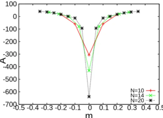
These relations mean that ϵ⁽⁴⁾(N, m) is N² times as large as ϵ^′′(N, m). The anomaly of A appears stronger than that of χ⁻¹ in the thermodynamic limit. In addition, from Eq. (3.16), the behavior ofϵ⁽⁴⁾(N, m)at m = 0andm = 1/N is different. Thus, we introduceAas physical concept for observing an anomaly.

Next, we discuss the case in whichϵ(m)is not analytic. ϵ(m)is not analytic for m when ϵ^′′(N, m) or ϵ⁽⁴⁾(N, m) diverges. In the thermodynamic limit, the relation is given by









 lim

N→∞ϵ^′′(N, m) =ϵ^′′(m)

⇒ϵ(m)is analytic,

Nlim→∞ϵ^′′(N, m) =±∞

⇒ϵ(m)is not analytic.

(3.17) (3.18)

The same holds for ϵ⁽⁴⁾(N, m). The divergence of ϵ^′′(N, m) and ϵ⁽⁴⁾(N, m) is equivalent to the fact thatχ⁻¹andAdiverge.

3.3 Free boson

We introduce the free boson which indicates the critical phenomena of the S = 1/2XXZ antiferromagnetic chain. The basics of conformal ﬁeld theory is introduced in AppendixD. First, for simplicity, we consider a free boson ﬁeldX(z, z) and an actionS.

S = 1 4πα^′

Z

d²x(∇X)² = 1 4πα^′

Z

d²x ∂X

∂x₁ 2

+ ∂X

∂x₂ 2!

= 1 4πα^′

Z

d²x[(∂zX+∂zX)² −(∂zX−∂zX)²]

= 1 πα^′

Z

d²z∂zX∂zX, (3.19)

(28)

whereα^′ is parameter which has lengthL²dimension,z =x₁+ix₂, z =x₁−ix₂,

∂z ≡ ¹₂(∂x₁ −i∂x₂), ∂z ≡ ¹₂(∂x₁ +i∂x₂), and d²x = ^dz_2i^∧^dz ≡ d²z. From an Euler-Lagrange equation, we obtain

∂z∂zX = 0. (3.20)

From Eq. (3.20), X(z, z) is a function ofz or z. Therefore, the free boson ﬁeld X(z, z)is divided into holomorphic part and antiholomorphic part.

X(z, z) =X(z) +X(z), (3.21) whereX(z)is a left-mover andX(z)is a right-mover.

Next, we consider a two-point correlation function. The two-point correlation function of the physical quantityx, x^′is given:

⟨x_qx_r⟩=A⁻_qr¹ ≡G_rq → Z

dxA(x, x^′)G(x^′) = δ(x−x^′), (3.22) whereGrqandG(x^′)are Green function andAqrandA(x, x^′)is the term involved in a gauss integral:

Z

dxexp

−1 2

txAx

= (2π)^N²(detA)⁻¹², (3.23) whereAis matrix andxis vector. The term corresponding toA_qr in the actionS is∂z∂z. Thus, the correlation function of the ﬁelds is derived from

⟨X(z, z)X(ω, ω)⟩= 1 Z

Z

X(z, z)X(ω, ω)e⁻^S(X⁾

= 1 2

− 1 πα^′∂z∂z

₋₁

δ(z−ω, z−ω)

∂z∂z⟨X(z, z)X(ω, ω)⟩=−πα^′

2 δ(z−ω, z−ω), (3.24)

whereZ is a partition function. The formula of Green function in two dimension is written in the form

∆ ln|z|= 4∂z∂zln|z|= 2πδ²(z, z), (3.25) whereδ²(z, z) =δ(z)δ(z). Comparing Eq. (3.24) with Eq. (3.25), we obtain

∂z∂z⟨X(z, z)X(ω, ω)⟩=−πα^′

2 δ(z−ω, z−ω)

=−α^′

2∂z∂zln|z−ω|².

(29)

Thus, the two-point correlation function ofX(z, z)andX(ω, ω)is

⟨X(z, z)X(ω, ω)⟩=−α^′

2 ln|z−ω|²

=−α^′

2 ln (z−ω)− α^′

2 ln (z−ω). (3.26) From Eq. (3.21), the two-point correlation function ofX(z)andX(z)is

⟨X(z)X(ω)⟩=−α^′

2 ln (z−ω),⟨X(z)X(ω)⟩=−α^′

2 ln (z−ω). (3.27) Subsequently, it is convenient to deﬁne the currentJ(z)as

J(z)≡ 2

α^′ 1/2

i∂zX(z). (3.28)

The product ofJ(z)is written in the form J(z)J(ω) = −

2 α^′

∂z∂ωX(z)X(ω)≃ 1

(z−ω)². (3.29) UsingJ(z), a stress-energy tensorT(z)which means Noether’s current is

T(z) = 1

2 :J(z)J(z) :≡ 1 2 lim

ω→z

J(ω)J(z)− 1 (z−ω)²

. (3.30)

The sign ‘: :’ is a normal order product where the annihilation operator is aligned to the right of the generation operator. For convenience, the currentJ is expanded for a Laurent expansion.

J(z) = 2

α^′ 1/2

i∂zX(z) = α₀z⁻¹+X

n̸=0

α_nz⁻ⁿ⁻¹ =X

n∈Z

α_nz⁻ⁿ⁻¹. (3.31) Similarly, the ﬁeldX(z)is derived:

X(z) = α^′

2

1/2"

ϕ₀−iα₀lnz+iX

n̸=0

α_n n z⁻ⁿ

#

, (3.32)

whereϕ₀is a zero mode. We then derive a commutation relation of the expansion coefﬁcientαn. Usingαn =H _dz

2πizⁿJ(z), we obtain the following relation [α_m, α_n] =

I dz

2πiz^mJ(z), I dω

2πiωⁿJ(ω)

=i² I

|z|>|ω|

dz

2πiz^m∂zX(z) I

ω=0

dω

2πiωⁿ∂ωX(ω)

−i² I

|z|<|ω|

dω

2πiωⁿ∂ωX(ω) I

z=0

dz

2πiz^m∂zX(z)

=mδ_m+n,0, (3.33)

量子スピン系における磁化率の異常に関する研究