Coupling of vortex breakdown and stability in a swirling flow
Author San To Chan, Jesse T. Ault, Simon J. Haward, E. Meiburg, Amy Q. Shen
journal or
publication title
Physical Review Fluids
volume 4
number 8
page range 084701
year 2019‑08‑15
Publisher American Physical Society
Rights (C) 2019 American Physical Society Author's flag publisher
URL http://id.nii.ac.jp/1394/00001043/
doi: info:doi/10.1103/PhysRevFluids.4.084701
Creative Commons Attribution 4.0 International (https://creativecommons.org/licenses/by/4.0/)
Coupling of vortex breakdown and stability in a swirling flow
San To Chan,1,*Jesse T. Ault,2,*Simon J. Haward,1E. Meiburg,3and Amy Q. Shen 1,†
1Okinawa Institute of Science and Technology Graduate University, Onna, Okinawa 904-0495, Japan
2Biomedical Sciences, Engineering, and Computing Group, Oak Ridge National Laboratory, Oak Ridge, Tennessee 37831, USA
3Department of Mechanical Engineering, University of California, Santa Barbara, Santa Barbara, California 93106, USA
(Received 5 April 2019; published 15 August 2019)
Swirling flows are ubiquitous over a large range of length scales and applications including micron-scale microfluidic devices up to geophysical flows such as tornadoes.
As the viscous dissipation, shear, and centrifugal stresses interact, such flows can often exhibit unexpected fluid dynamics. Here, we use microfluidic experiments and numerical simulations to study the flow in a vortex T-mixer: a T-shaped channel with staggered, offset inlets. The vortex T-mixer flow is characterized by a single dominant vortex, the stability of which is closely coupled to the appearance of vortex breakdown. Specifically, at a Reynolds number of Re≈90, a first vortex breakdown region appears in the steady-state solution, rendering the vortex pulsatively unstable. A second vortex breakdown region appears at Re≈120, which restabilizes the vortex. Finally, a third vortex breakdown region appears at Re≈180, which renders the vortex helically unstable. Thus, a counterintuitive flow regime exists for the vortex T-mixer in which increasing the Reynolds number has a stabilizing effect on the steady-state flow. The pulsatively unstable vortex evolves into a periodically pulsating state with a Strouhal number of St≈0.5, and the helically unstable vortex evolves into a helically oscillating state with St≈1.75. These transitions can be explained within the framework of linear hydrodynamic stability. In addition, the vortex T-mixer flow exhibits multistability; multiple flow states are stable over various ranges of Re, including a narrow range of tristability for 160Re170, in which the steady state, the pulsatile oscillation, and the helical oscillation are all stable. This study provides experimental and numerical evidence of the close coupling between vortex breakdown and flow stability, including the restabilization of the flow with increasing Reynolds number due to the appearance of a vortex breakdown region, which will provide new insights into how vortex breakdown can affect the stability of a swirling flow.
DOI:10.1103/PhysRevFluids.4.084701
I. INTRODUCTION
Swirling flows are flows which rotate about an axis; a typical example is tornado. They exhibit a diverse range of fluid dynamical behaviors as the viscous dissipation, shear, and centrifugal stresses interact. For instance, strong enough centrifugal stress can trigger a phenomenon called vortex
*Authors contributed equally to this work.
Published by the American Physical Society under the terms of the Creative Commons Attribution 4.0 Internationallicense. Further distribution of this work must maintain attribution to the author(s) and the published article’s title, journal citation, and DOI.
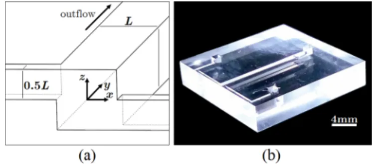
FIG. 1. Microfluidic T-mixer with staggered, offset inlets (vortex T-mixer). (a) Coordinate system and schematic of the vortex T-mixer. (b) Experimental devices are fabricated in glass using a LightFab 3D-printer.
Both inflows enter the junction tangentially, resulting in the development of a swirling flow characterized by a single, dominant vortex structure.
breakdown, which corresponds to the sudden structural change of the vortex core of a swirling flow; for example, the sudden divergence of stream surfaces [1,2].
Two predominant types of vortex breakdown exist: the bubble-type and the spiral-type [3].
Bubble-type breakdown is characterized by a nominally axisymmetric flow recirculation zone that is bounded by upstream and downstream internal stagnation points. If a tracer filament is injected on the vortex axis, then it will become trapped in the recirculation zone and appear like a bubble [4]. Spiral-type breakdown is instead characterized by a single internal stagnation point followed by a helical motion of the vortex core downstream. In this case, a tracer filament will kink at the location of the stagnation point and flutter helically downstream [5]. Spiral-type breakdown can be further characterized into the single and double forms. The single form has only one fluttering helix while the double form has two. Direct numerical simulations [6–8] have revealed that spiral-type breakdown is caused by a large pocket of absolute instability that is located around the bubble-type breakdown region. Thus, the bubble-type is the more basic form of vortex breakdown.
Both types of vortex breakdown are of vital importance to the understanding of natural phenom- ena and to the performance of engineering systems. For example, vortex breakdown observed in model tornadoes plays a crucial role in inferring the internal structure and evolution of real tornadoes [9,10]. In combustion systems, recirculation zones due to bubble-type breakdown can help fuels burn more effectively and create a compact, stable flame [11–13]. In aerodynamics systems, such as flow over a delta wing, depending on the angle of attack, breakdown can occur in the leading-edge vortices, which can drastically alter stability of the aircraft [14,15]. Recently, vortex breakdown has seen applications in microfluidics due to its ability to manipulate microparticles in a branching T-junction flow [16–21], in which one inflow splits into two opposite outflows.
Here, we combine microfluidic experiments and numerical simulations to study the mixing flow in a T-shaped channel with staggered, offset inlets, which we will refer to as a vortex T-mixer (Fig.1). This flow geometry was chosen for two main reasons. First, unlike the branching T-junction flow which has four Dean vortices [16–21], the vortex T-mixer flow has only one single dominant vortex, which greatly simplifies the interpretation of the numerical and experimental results. Second, it is easy to perform measurements for the vortex T-mixer flow. For instance, the flow field can be quantitatively measured directly at the channel cross-section, allowing direct comparison between the experimental and numerical results.
We will show that the vortex T-mixer flow exhibits stability characteristics that are tightly coupled to the appearance and evolution of vortex breakdown regions. In particular, at a Reynolds number (which quantifies the relative inertial and viscous effects of a flow) of Re≈90, a single bubble-type vortex breakdown region appears in the steady-state flow. The appearance of this region destabilizes the flow to pulsative perturbations and triggers the transition of the steady-state flow to a stable periodically pulsating state with a Strouhal number (which is the dimensionless frequency of an
oscillation) of St≈0.5. At Re≈120, a second vortex breakdown region appears that restabilizes the steady-state flow. Thus, the vortex T-mixer flow exhibits counterintuitive stability characteristics in this Reynolds number range in which increasing the Reynolds number actually has a stabilizing effect on the flow. Finally, a third vortex breakdown region appears at Re≈180 that renders the flow unstable to helical perturbations, triggering the steady state to undergo spiral-type breakdown and resulting in a stable helical oscillating state with St≈1.75. In addition, the vortex T-mixer flow shows a strong history dependence. That is, depending on how Re is varied, multiple flow states can be stable over different Re ranges, including a narrow range of 160Re170 in which the steady, pulsatile, and helical states are all stable.
In the following sections we present experimental and numerical evidence of this close coupling between the formation of vortex breakdown in the vortex T-mixer and the stability characteristics of the flow, which will point to new research directions for the study of vortex breakdown. In Sec.IIwe describe the experimental and numerical methodologies used in this analysis, in Sec.IIIwe present results and discussion, and in Sec.IVwe present conclusions and ideas for future work.
II. METHODOLOGY
In this section, we describe the experimental methodology used to fabricate our devices and perform the experiments, we introduce the notations that will be used throughout, and we describe the numerical approach used to simulate the T-mixer flow.
A. Microfluidic device
All experiments were performed in a vortex T-mixer as shown in Fig.1(a). This channel geometry contains aZ2symmetry [22], as it is invariant to a rotation of angleπabout theyaxis. The choice to offset the inlets in this geometry was originally proposed as an approach to enhance the mixing performance of a simple T-shaped microchannel [23,24]. In this vortex T-mixer, both inflows enter the outlet channel tangentially, resulting in a swirling flow characterized by one dominant vortex structure that decays downstream in the outlet channel.
The vortex T-mixer was fabricated in glass using a LightFab 3D printer (LightFab GmbH, Germany), which utilizes selective laser-induced etching (SLE) technology [25,26]. The LightFab 3D printer employs ultrafast laser pulses to print channels inside a piece of fused silica. The channels are then etched with potassium hydroxide (KOH) in an 80◦C ultrasonic bath at an approximate rate of 100μm/h. Etching of the channels is about 1000 times faster than that of the bulk glass. The final product is a transparent, rigid piece of glass with embedded channels that can endure both organic solvents and high pressure [see Fig. 1(b)]. Four of the six outer surfaces of the etched device are opaque; however, optical access can be gained by adding a thin film of water onto those surfaces. The outlet channel has a length of 20 mm and a square cross-section with side lengths ofL=1±0.06 mm. A brief numerical study was performed to confirm that this outlet channel is sufficiently long such that the flow is insensitive to the outlet conditions [27,28]. The inlet channels have square cross-sections with side lengths of 0.5±0.01 mm and lengths of 8 mm, which ensures that the flow is fully developed before reaching the junction.
B. Notations
Here, we briefly summarize our notations. We define the Reynolds number as Re=U L/ν, where U is the mean flow speed in the outlet channel,νis the kinematic viscosity of the fluid, andLis the side length of the outlet channel. The coordinates, flow velocities, and time are nondimensionalized by L,U andL/U, respectively. Those dimensionless variables are denoted asx=(x,y,z),u= (ux,uy,uz) and t. For flows that oscillate periodically, the Strouhal number St= f L/U is used to nondimensionalize the oscillation frequency f. The term flow staterefers to the set of flows that persist over a particular set of Re and for which the flow oscillation can be approximately characterized by a single St.
C. Flow-rate control
The flow was driven by three individually controlled neMESYS syringe pumps (Cetoni GmbH, Germany) equipped with 25-ml glass syringes (Hamilton Gastight, Reno, NV). The pumps operate at a minimum of 5× (typically 50×) the specified pulsation-free flow rate to eliminate pump- induced vibrations. The microfluidic device and syringes were connected by rigid polyethylene tubing to minimize hydraulic compliance. As the flow state depends on how Re is varied, two different approaches were used to initialize a desired Re in an experiment. The first is to directly increase Re from zero to the desired value in approximately 0.1 s, which corresponds to a dimensionless rate of O(10). The second is to slowly vary Re at a rate of approximately 1 s−1, which corresponds to a dimensionless rate ofO(0.01), from a reference value Re1 to the desired value Re2. With these two different initialization strategies we can demonstrate the multi-stability in which multiple stable solutions exist for a given Re.
D. Fluorescent dye visualization
Fluorescent dye visualization was performed on the outlet channel cross-section aty=2. To achieve this, one of the T-mixer inflows was supplied with pure water, while the other was supplied with a 0.05 g/L sodium fluorescein solution. A metal hallide lamp with a 488 nm excitation filter illuminated the channel, inducing fluorescence of the fluorescein-dyed fluid. Videos of the dye ad- vection patterns under flow at various Re were captured by an inverted microscope (Nikon ECLIPSE Ti) equipped with a spinning-disk confocal imaging system (DSD2, Andor Technology Ltd) and a 0.10 NA, 30 mm WD, and a 4×objective (Nikon CFI Achro 4X) with an exposure time of 20 ms.
E. Microparticle image velocimetry (μPIV)
Time-resolved microparticle image velocimetry (μPIV) [29] was performed on the outlet channel cross-section aty=2. Red fluorescent polystyrene particles of diameter 2μm and density 1.05 g/cm3were seeded in deionized water and illuminated by a 527-nm dual-pulsed Nd:YLF laser (Terra PIV, Continuum Inc., CA) with an average power of 60 W and a pulse durationδt <10 ns.
Depending on the considered Re, the laser repetition ranged from 500 to 1630 Hz, and the time separation between two laser pulses ranged from 5 to 100 μs. TheμPIV images were captured by an inverted microscope (Nikon ECLIPSE Ti-S) equipped with a 1280×800 pixels high-speed CMOS camera (Phantom Miro M310, Vision Research Inc., NJ) and a 0.15 NA, 23.5 mm WD, 5×objective (Nikon CFI Plan Fluor 5X). The measurement depth [30] over which the fluorescent particles contribute to the determination of the flow field was approximately 0.1L. To accurately compute St for the flow oscillation, at least 400 μPIV images were captured for each Re. Dye visualization videos were also captured by the same high speed camera at 4 000 and 10 000 Hz to ensure that theμPIV measurements satisfied the Nyquist-Shannon sampling criterion [31].
F. Numerical simulation
Simulations were performed using the open source computational fluid dynamics software OpenFOAM [32]. Steady-state simulations were performed using the built-in solversimpleFoam, and transient simulations were performed using a modified version of theicoFoamsolver. Fully developed inlet velocity profiles were implemented using thegroovyBCboundary condition utility provided by the swak4Foam package, which corresponds to the experimental inflow condition.
The selected solvers are second-order accurate in both space and time. A simulation domain that corresponds to the microfluidic device was generated using the built-in blockMesh utility. All simulations were performed using the same mesh with inlet channels of length 4L and an outlet channel of length 15L. The outlet channel was determined to be sufficiently long such that the fluid dynamics of the system is insensitive to the outlet boundary condition [27,28], and the outflow is approximately fully developed up to the maximum Re used in this study, which corresponds to the experimental outflow condition.
The boundary conditions imposed on the fluid velocity include a fully developed inflow condition at each channel inlet, no-slip conditions on all channel walls, and a zero-normal-gradient condition at the channel outlet. This implicitly assumes that the flow is fully developed when it reaches the channel outlet. Boundary conditions on the fluid pressure were selected to be zero-normal-gradient at the channel inlets and at the channel walls, as well as a fixed uniform outlet pressure of p=0.
This inlet boundary condition on the pressure, while not analytically correct, is helpful for the stability of the solvers, and the errors introduced by it are confined to a narrow region within one or two cell lengths of the channel inlets. Additional descriptions of the simulation domain, mesh design and inflow condition, as well as the results of a numerical convergence study are presented in AppendixA.
G. Stability of steady-state solutions
Steady-state simulations were performed for Re ranging from 10 to 250 by increments of 10.
Residual tolerances were set to 10−6for both the fluid pressure and velocity; relaxation factors of 0.3 and 0.7 were respectively chosen for the pressure and velocity. Using this setup, the steady-state solutions up to Re=220 successfully converged in less than one hour while running on 64 cores on the Titan supercomputer. These simulations were initialized using initial conditions of u=0 and p=0 everywhere. To test the flow stability, converged steady-state solutions were imported as initial conditions into a transient solver. These simulations were carried on until velocity measurements at probed locations were confirmed to be steady or until they achieved stable periodic orbits. Subsequently, additional simulations were performed to determine the Re limits of transition between states using the steady-state and the stable oscillating solutions as initial conditions with incrementally varied Re until a new periodic orbit was achieved or the flow transitioned back to steady.
III. RESULTS AND DISCUSSIONS A. Unstable-stable transition
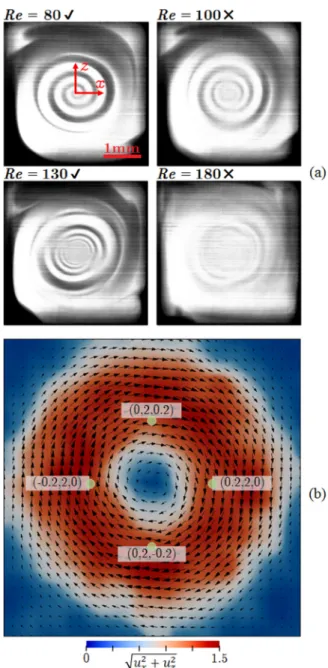
To motivate a systematic analysis of the fluid dynamics in a vortex T-mixer, we first present an unexpected experimental observation that for the same geometry and with steady inlet conditions, the laminar steady-state base flow, which is unstable for approximately 80<Re<120, can be restabilized by increasing the Reynolds number. Experimentally, this effect was observed using dye visualizations as described in the previous section and initializing the flow rate on the syringe pumps directly to the target Reynolds number. For each Re, a dye visualization video with at least 100 frames was time-averaged to form a single image as shown for Re=80, 100, 130, and 180 in Fig.2(a).
For steady-state flows, the time-averaged dye visualization should contain a clear interface between the two inflows of water and dye, whereas for unsteady flows this interface will be blurry due to the averaging over the video frames. In Fig. 2(a)we see that for Re=80, a spiral with clear winding can be observed at the channel center, signifying a steady flow. The handedness of the spiral is solely determined by thez-offset of the two inlet channels and is hence independent of the initial condition applied. Increasing the Reynolds number to Re=100, the spiral blurs out, suggesting that the flow has transitioned to unsteady. Surprisingly, at Re=130 a clear spiral is once again observed, suggesting that the flow has regained its steadiness. Finally, at Re=180 the spiral almost completely disappears as the flow transitions back to unsteady once again. Thus, the vortex T-mixer flow demonstrates a counter-intuitive flow regime within which increasing the Reynolds number can restabilize the steady-state base flow. A video corresponding to the results presented in Fig.2(a)can be found in the Supplemental Material [33].
FIG. 2. Example experimental results on the channel cross-sectiony=2. (a) Time-averaged fluorescent dye visualizations at different Reynolds numbers. A clear spiral between the two inflows of water and dye indicates a steady flow, as labeled by check marks, and a blurry spiral indicates an unsteady flow, as labeled by a cross. A corresponding video can be found in the Supplemental Material [33]. (b) A snapshot of the time-resolved microparticle image velocimetry (μPIV) results at Re=100.
B. St-Re flow state diagram
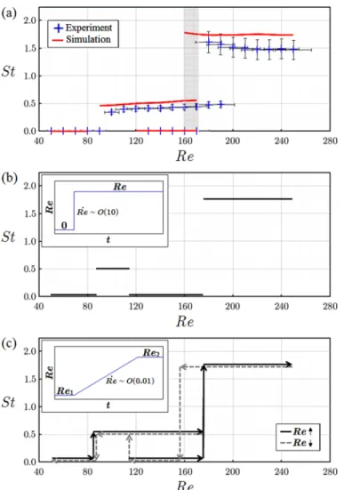
Motivated by the experimental observation of this unexpected restabilization, we performed a systematic experimental and numerical study of the different flow regimes, stability characteristics, and flow transitions observed in the vortex T-mixer flow. These results can be summarized in a St-Re state diagram as shown in Fig.3. For each Re, the Strouhal number was obtained from a time series
FIG. 3. St-Re flow state diagram. (a) Strouhal number St as a function of Re. Experimental and numerical results are respectively labeled as blue crosses and red lines. The vortex T-mixer flow can be characterized into three states, with St=0, St≈0.5 and 1.75. (b) A schematic showing how the flow state changes when Re is directly increased from zero to the desired value. (c) A schematic showing how the flow state changes when Re is varied from a reference value Re1to a desired value Re2linearly at a slow rate. Black solid and gray dashed arrows respectively indicate the increasing and decreasing of Re.
ofuzprobed at the locationx=(0,2,0.2). These results were obtained using both time-resolved μPIV [Fig. 2(b)] and transient simulations as described in the methodology section. Figure3(a) shows the experimentally and numerically observed Strouhal numbers for the vortex T-mixer flow as a function of Re. Figure3(b)shows the flow state that is achieved when the flow rate is directly increased from zero to the target Reynolds number, while Fig. 3(c) shows the flow state that is achieved when the Reynolds number is gradually varied at a slow rate.
The St-Re state diagram shown in Fig.3 illustrates three distinguishing features of the vortex T-mixer flow. First, the vortex T-mixer flow can be characterized into three states, each of which has a distinct St, as shown by the four nominally horizontal red lines obtained by simulation in Fig.3(a).
The steady-state solution with St=0 is seen to be stable for 0Re80 and 120Re170, the St≈0.5 state is stable for 90Re170, and the St≈1.75 state is stable for Re160. Second, the vortex T-mixer flow exhibits multistability, that is, within certain Re ranges multiple flow states
are stable, including a region of tristability. This regime appears in the Reynolds number range 160 Re170, where the steady St=0 state, the St≈0.5 state, and the St≈1.75 state are all stable. This is illustrated by the gray shaded area in Fig.3(a).
Finally, the St-Re state diagram illustrates the history-dependence, i.e., hysteresis, of the vortex T-mixer flow as the Reynolds number is varied. When the flow rate is initialized directly to achieve the desired Reynolds number, a single flow state exists for each Re as shown in Fig.3(b). Similarly, if the numerically obtained steady-state solutions are used as initial conditions in a transient solver, then the flow will transition to the St≈0.5 state for 90 Re110 and will remain in the steady state for 120 Re170. However, if Re is increased or decreased slowly from a reference value Re1to the desired value Re2as shown in Fig.3(c), then the flow states can persist for larger ranges of Re, giving rise to the multistability. For example, slowly increasing Re for the St≈0.5 state can preserve this state up to Re≈170.
In the next sections, we will take an in-depth look at the three different identified flow states and elucidate the connection between the appearance of vortex breakdown regions and the dynamical shifts in stability of the flow.
C. The St≈0.5 state
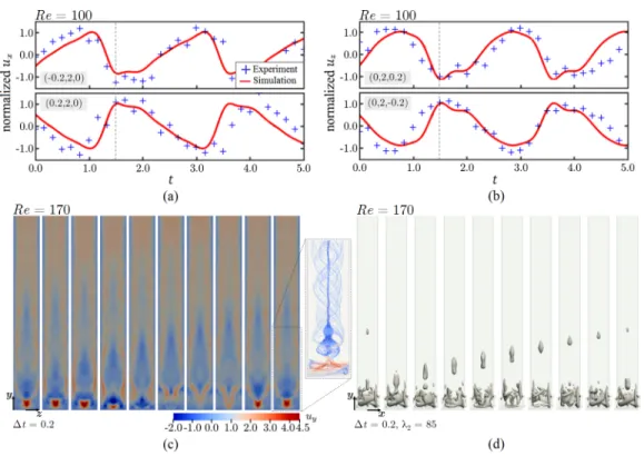
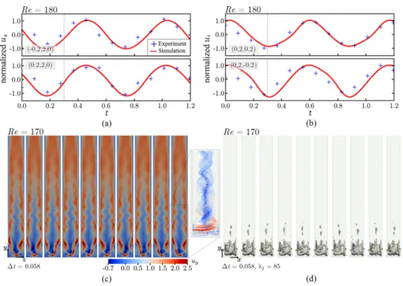
First, we consider dynamics of the St≈0.5 state. Representative experimental and numerical results characterizing this flow state are shown in Fig.4for (a, b) Re=100 and (c, d) Re=170.
Time series data ofuxatx=(−0.2,2,0) and (0.2, 2, 0), anduzatx=(0,2,0.2) and (0,2,−0.2) are presented in Figs.4(a)and4(b). These locations correspond to the left, right, top and bottom sides of the channel cross-section aty=2. As can be seen,uxoscillates out-of-phase on the left and right sides of the channel [Fig.4(a)], anduz oscillates out-of-phase on the top and bottom sides of the channel [Fig.4(b)]. The right/left oscillations are seen to be out-of-phase with the top/bottom oscillations. Essentially, the flow is undergoing a nonaxisymmetric, pulsatile motion analogous to the compressing and stretching of a hula hoop along one direction, which preserves theZ2symmetry of the vortex T-mixer. As can be seen, there is close agreement between the numerical simulations and the experimentalμPIV results.
To enable direct comparison between the different flow states, we also present detailed numerical results for the case of Re=170 at which the flow exhibits tristability. This will allow us to compare the steady-state flow, the pulsating St≈0.5 flow, and the helically oscillating St≈1.75 flow under identical inflow conditions. Distributions of the axial velocity uy on the channel midplanex=0 are shown in Fig.4(c) as a function of time. As the St≈0.5 state preserves theZ2 symmetry, distributions ofuyonx=0 are symmetric about thez=0 plane. In addition, bubble-type vortex breakdown is evidenced by a recirculation zone as shown by the 3D streamline visualization on the right side of Fig.4(c). Figure4(d)shows a level set of theλ2 criterion, which is an algorithm for identifying vortices from three-dimensional velocity fields [34,35]. Here,λ2=85. The results in Figs. 4(c)and4(d)both correspond to approximately one full period of the stable oscillation.
In each oscillation a single pocket of recirculating flow (i.e., a vortex breakdown bubble) is generated in the junction and then advected downstream, where it ultimately decays due to viscous dissipation.
D. The St≈1.75 state
Next, we perform a similar characterization of the flow for the St≈1.75 state and compare it with the pulsating state. Representative experimental and numerical results characterizing this flow state are shown in Fig.5for (a, b) Re=180 and (c, d) Re=170. Once again, we consideruxat x=(−0.2,2,0) and (0.2, 2, 0) anduzatx=(0,2,0.2) and (0,2,−0.2) and we plot the time series data in Figs.5(a)and5(b). In contrast to the pulsating St≈0.5 state, hereux oscillates in-phase on the left and right sides of the channel [Fig.5(a)], as doesuz on the top and bottom sides of the channel [Fig.5(b)]. Furthermore, the right/left oscillations here have a phase difference ofπ/2 with
FIG. 4. The St≈0.5 state. (a) Flow velocityuxoscillating out-of-phase at locationsx=(−0.2,2,0) and (0.2, 2, 0). (b) Flow velocityuzoscillating out-of-phase at locationsx=(−0.2,2,0) and (0.2, 2, 0). The four locations correspond to the left, right, top and bottom sides on the channel cross-section aty=2. Blue crosses and red lines represent the experimental and numerical results, respectively. Panels (a) and (b) are results with Re=100 and show that the flow is undergoing a nonaxisymmetric pulsatile motion, which is analogous to the compressing and stretching of a hula hoop along one direction. (c) Axial velocityuyon the channel mid- planex=0. Distributions ofuyare symmetric across thez=0 plane. The dashed box contains representative 3D streamlines that show a recirculation zone developing in the junction, which signifies bubble-type vortex breakdown. (d) A level set of theλ2criterion [34,35] withλ2=85. As can be seen, through each oscillation, a pocket of bubble-type vortex breakdown develops in the junction which is advected downstream where it ultimately decays. Panels (c) and (d) are results with Re=170 and represent approximately one full cycle of the pulsatile motion witht=0.2 between frames. A corresponding video can be found in the Supplemental Material [33].
the top/bottom oscillations. Thus, the flow is undergoing a periodic oscillating helical motion in the outlet channel, which breaks theZ2symmetry of the vortex T-mixer flow.
As with the pulsating state, the experimental and numerical results show good agreement. To facilitate direct comparison between the two oscillating states, we again include detailed numerical results for Re=170 that falls within the regime of tristability. Figure 5(c) shows the evolution of uy on the x=0 channel center plane throughout a single complete oscillation of the flow.
Unlike the St≈0.5 state, here the oscillation clearly arises from a symmetry-breaking instability as the distributions ofuyonx=0 are asymmetric about thez=0 plane. Within the junction, the vortex core is nominally axisymmetric, but this breaks down and the vortex oscillates helically downstream, as shown by the streamline visualization in Fig.5(c), signifying the onset of spiral-type vortex breakdown [3]. Finally, Fig.5(d)shows a level set of theλ2 criterion again withλ2=85.
These results clearly distinguish the dynamics of the vortex breakdown regions between the two oscillating states. Whereas with the pulsating St≈0.5 state the recirculation zone was produced in the junction and advected downstream along the outlet channel centerline, here several small
FIG. 5. The St≈1.75 state. (a) Flow velocityux oscillating in-phase at locationsx=(−0.2,2,0) and (0.2, 2, 0). (b) Flow velocityuz oscillating in-phase at locationsx=(−0.2,2,0) and (0.2, 2, 0). The four locations correspond to the left, right, top and bottom sides on the channel cross-section aty=2. Blue crosses and red lines represent the experimental and numerical results, respectively. Panels (a) and (b) are results with Re=180 and show that the left/right oscillations have a phase difference ofπ/2 with the top/bottom oscillations, signifying that the flow is undergoing a periodic helical oscillation. (c) Axial velocityuyon the channel mid-planex=0. Distributions ofuyare asymmetric over thez=0 plane. The dashed box contains representative 3D streamlines that show that the vortex core is nominally axisymmetric in the junction but undergoes nonaxisymmetric helical motion downstream, signifying the onset of spiral-type vortex breakdown.
(d) A level set of theλ2criterion [34,35] withλ2=85. As can be seen, within the junction a single pocket of vortex, corresponding to the nominally axisymmetric vortex core, rotates around its own axis at a fixed position in the junction. Downstream, several small pockets of vortex helically oscillate about the channel centerline.
Panels (c) and (d) are results with Re=170 and represent approximately one full cycle of the helical oscillating motion witht=0.058 between frames. A corresponding video can be found in the Supplemental Material [33].
pockets of recirculation appear to oscillate around the outlet channel centerline within a narrow range approximately 1.5Lto 2.5L from the channel bottom. Furthermore, the breakdown does not appear to have any rotational symmetries, suggesting that the spiral-type vortex breakdown seen here is of the single form.
E. The steady St=0 state
As we have shown, the steady-state flow, the pulsating St≈0.5 flow, and the helically oscillating St≈1.75 states are all stable solutions within the range of tristability given by 160 Re170.
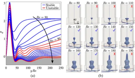
This suggests that the St≈0.5 and 1.75 states arise from the steady-state base flow through different instability mechanisms. To elucidate these instability mechanisms, we consider the evolution of the steady-state base flow as a function of Reynolds number, and we especially emphasize
FIG. 6. Stability of the steady-state solutions. (a) Distributions of dimensionless axial velocity uy of the steady-state solutions along the channel centerline. Increasing Re changes the curvature and level of uy=uy(yRe), which in turn changes the number and positions of the internal stagnation points. (b) 3D streamline visualizations of the vortex breakdown regions in the outlet channel as a function of Re. The first bubble-type vortex breakdown region appears at around Re=90. A second region then appears downstream of the first one at around Re=120. These merge and become a single larger structure at around Re=130.
Finally, a third region appears further downstream at around Re=180 and enlarges and slenderizes the aforementioned second breakdown region. Blue check marks indicate stable solutions and red crosses indicate unstable solutions. Thus, the appearance of each subsequent vortex breakdown region results in a dynamical shift in the stability of the base state. That is, with zero vortex breakdown regions the flow is stable. When the first breakdown region appears, the flow becomes unstable. When the second breakdown region appears, the flow is restabilized. Finally, when the third breakdown region appears, the flow becomes unstable again.
To the best of our knowledge, this is the first example of a flow in which the stability of the flow is so closely coupled to the appearance and dynamics of vortex breakdown.
the qualitative dynamical shifts that occur which are characterized by the appearance of vortex breakdown regions.
A summary of this systematic investigation of the steady-state base flow showing the outlet centerline axial velocity component, streamline representations of the vortex breakdown regions, and the stability classification for a range of Reynolds numbers is presented in Fig.6. Specifically, Figure 6(a) shows how the dimensionless axial velocity component uy varies along the outlet channel centerline for 30 Re190. Here,uyis plotted againstyRe for visualization purposes;
doing so nicely collapses the data by effectively aligning the peaks of uy. Vortex breakdown is indicated by the regions in whichuy<0 and is represented by the solid gray box. As can be seen, starting from Re=30, increasing Re results in a local minimum ofuythat first goes negative around Re=90, representing the onset of vortex breakdown. Varying the Reynolds number also results in a qualitative dynamical shift in the number of internal stagnation points. For example, for Re80, there are no internal stagnation points. However, at Re=90, there are two internal stagnation points, also signifying the onset of bubble-type vortex breakdown.
Corresponding to the results in Fig. 6(a), 3D streamline visualizations of vortex breakdown regions in the outlet channel are shown as a function of Re in Fig. 6(b). They appear similar to those observed in a cylinder with a rotating end wall [36–38], which is a classical system for studying bubble-type vortex breakdown. At around Re=90, a first bubble-type vortex breakdown region appears. Around Re=120, a second region appears downstream of the first. As the Reynolds number increases further, these regions merge at around Re=130. Finally, a third vortex breakdown
region appears around Re=180, enlarging and slenderizing the aforementioned second breakdown region. This region also merges into the existing breakdown structure at a slightly higher Reynolds number.
F. Stability of the steady-state solutions
Finally, we consider the stability and transient evolutions of the steady-state base flow solutions, we document the instability mechanisms that trigger transition, and we emphasize the close connection between the stability and vortex breakdown characteristics for the vortex T-mixer. First, we test the stability of each of the steady-state solutions as described in the methodology section, the results of which are shown in Fig.6. As can be seen, every qualitative dynamical shift in the stability of the base state corresponds to a qualitative shift in the vortex breakdown characteristics of the flow. The base state is stable up until around Re=90, where the first vortex breakdown region appears, triggering a pulsative instability in the vortex that causes a transition to the pulsating St≈0.5 state. At around Re=120, the second vortex breakdown region appears, which restabilizes the steady-state flow solution. At around Re=180, the third vortex breakdown region appears, triggering a helical instability in the vortex that causes a transition to the helically oscillating St≈1.75 state. Thus, in the vortex T-mixer flow, stability characteristics of the flow are intimately coupled with the emergence and evolution of vortex breakdown. To the best of our knowledge, this is the first instance where this relationship has been identified to such a convincing extent.
Next, we seek to identify how and where the fluctuations grow on the steady-state solutions.
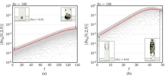
To achieve this, we probe the fluctuating velocity component|δuz| = |uz(x,t)−uz(x,0)|at x= (0,2,0) as a function of time; for a linear instability, this perturbation velocity component should grow roughly exponentially over time. We also identify the location where the fluctuation originates by visualizing a level set of|δu| = |u(x,t)−u(x,0)|. For the pulsating and helically oscillating states, we report results for the cases of Re=100 and 180, respectively, which are unstable according to Fig.6.
Results presenting the exponential growth of the fluctuating velocity components and the visualizations of the origins of the fluctuations are shown in Fig.7. As can be seen, for both the pulsating and helically oscillating states, the perturbation velocity components grow exponentially in time, indicating that both states result from linear instabilities. For the Re=100 case, in which a single vortex breakdown bubble is present, the level set|δu| =0.01 appears within the junction of the vortex T-mixer, indicating that the fluctuation originates around the first vortex breakdown region. However, for the Re=180 case, in which three vortex breakdown regions are present, the level set|δu| =0.01 appears further downstream in the outlet channel, indicating that the fluctuation originates around the third vortex breakdown region. As this fluctuation grows, it extends upstream, suggesting that there is a pocket of absolute instability around the third vortex breakdown region.
This renders the steady-state solution globally unstable and triggers the helical St≈1.75 oscillation that corresponds to spiral-type vortex breakdown [6]. Numerical results visualizing the growth of both oscillating states with particle tracers are presented in AppendixB.
As a final point of analysis, we apply the method of Ruithet al.[6] to calculate the criticality of the base state and demonstrate that, as expected, the appearance of vortex breakdown in the vortex T-mixer does correspond to the appearance of a pocket of subcriticality. This procedure involves axisymmetrizing the vortex data near the vortex core within a region where the flow is nominally axisymmetric. For simplicity, we select a cylindrical region about the vortex core with radiusL/4.
Next, the velocity is expressed in cylindrical coordinates, and we seek solutions to the differential equation given by [6]
d2 dr2 −1
r d dr + 1
r3u2y d(ruθ)2
dr − r uy
d dr
1 r
duy
dr
φc=0,
FIG. 7. Instability on the steady-state solutions. (a) Growth of the St≈0.5 fluctuation at Re=100. The fluctuation|δuz| = |uz(x,t)−uz(x,0)|atx=(0,2,0) grows exponentially with timet, indicating that the St ≈0.5 state is the result of a linear instability. A level set|δu| = |u(x,t)−u(x,0)| =0.01 shows that the fluctuation originates around the first bubble breakdown region. (b) Growth of the St≈1.75 fluctuation at Re= 180. The fluctuation|δuz| = |uz(x,t)−uz(x,0)|atx=(0,2,0) grows exponentially with timet, indicating that the St≈1.75 state is also the result of a linear instability. A level set|δu| = |u(x,t)−u(x,0)| = 0.01 shows that the fluctuation originates around the third bubble breakdown region. When|δuz| reaches its plateau at sufficiently larget, the level set extends upstream, implying that there is a pocket of absolute instability around the third bubble breakdown region which generates the fluctuation.
subject to the boundary conditionsφc(0) =0 anddφc(0)/dr=1. Critical values are sought such that φc(rcrit)=0, and the procedure is repeated for each axial location along the outlet channel.
Finally, subcritical regions can be identified by plotting rcrit as a function ofyand comparing it with a certain threshold. Numerical results for our data are presented in Fig.8 for Re=60, 90, and 120, which correspond to Reynolds numbers for which we expect zero, one, and two vortex breakdown regions. As can be seen, for Re=90,rcrit →0 at the same axial location where the first vortex breakdown region appears, and for Re=120,rcrit →0 at approximately the same locations where the first two vortex breakdown regions appear. Despite the fact that several assumptions
FIG. 8. Numerical results computing the criticality of our flows using the approach presented by Ruith et al.[6]. As can be seen, the appearance of a pocket of subcriticality corresponds to the appearance of vortex breakdown. Results correspond to (a) Re=60, (b) Re=90, and (c) Re=120, for which we expect zero, one, and two regions of vortex breakdown in the flow. In each case, the axial locations where pockets of subcriticality appear correspond precisely with the locations of vortex breakdown.
of the original theory presented by Ruithet al.[6] are less valid for our specific data due to the combination of flow geometry and Reynolds numbers, nevertheless, the application of this approach and the interpretation of vortex breakdown as due to the appearance of a pocket of subcriticality appear to be well validated by this theory applied to the vortex T-mixer.
IV. CONCLUSIONS
The vortex T-mixer flow that we have studied here demonstrates several fluid dynamical features. We have identified a counter-intuitive flow regime in which increasing the Reynolds number restabilizes an unstable flow state. Crucially, this restabilization corresponds exactly to the appearance of a second vortex breakdown region that presumably restabilizes the flow via a mechanism related to the nonlinear vortex breakdown dynamics. More generally, we have shown how the development and evolution of vortex breakdown in the vortex T-mixer are exactly coupled with the stability characteristics of the flow. The appearance of the first vortex breakdown region around Re=90 triggers a pulsative instability in the flow that launches the growth of a St≈0.5 pulsating state. The appearance of a second vortex breakdown region around Re=120 restabilizes the base state. Finally, the appearance of a third vortex breakdown region around Re=180 triggers a helical instability in the flow that launches the growth of a helically oscillating St≈1.75 state.
Furthermore, the vortex T-mixer flow demonstrates flow regimes of multi-stability, including a regime of tristability for 160Re170 in which the steady, pulsating, and helically oscillating states are all stable. As future work, we plan to investigate in detail the specific mechanism by which the second vortex breakdown region stabilizes the flow using a global stability analysis.
Furthermore, preliminary simulations with a cylindrical outlet suggest that the role of the corners may play a key role in this restabilization. Finally, a third oscillating state with St≈3.0 was identified numerically, although its sensitivity to initial conditions prevented us from studying this state experimentally. We hope to improve the sensitivity of our experimental approach in the future to verify and study this state. Ultimately, the vortex T-mixer flow that we have described here has demonstrated novel fluid dynamical features, the most important to be the close coupling between the vortex breakdown phenomenon and the stability characteristics of the flow, which to the best of our knowledge has not been documented elsewhere.
ACKNOWLEDGMENTS
We gratefully acknowledge useful discussions with Prof. Howard A. Stone from Princeton University. S.T.C., S.J.H., and A.Q.S. acknowledge the support of the Okinawa Institute of Science and Technology Graduate University, with subsidy funding from the Cabinet Office, Government of Japan. S.J.H. and A.Q.S. also acknowledge funding from the Japan Society for the Promotion of Science (Grants No. 17K06173, No. 17J00412, No. 18K03958, and No. 18H01135). This manuscript has been authored by UT-Battelle, LLC under Contract No. DE-AC05-00OR22725 with the U.S. Department of Energy. The United States Government retains and the publisher, by accepting the article for publication, acknowledges that the United States Government retains a nonexclusive, paid-up, irrevocable, world-wide license to publish or reproduce the published form of this manuscript, or allow others to do so, for United States Government purposes. The Department of Energy will provide public access to these results of federally sponsored research in accordance with the DOE Public Access Plan (http://energy.gov/downloads/doe-public-access-plan). Research sponsored by the Laboratory Directed Research and Development Program of Oak Ridge National Laboratory, managed by UT-Battelle, LLC, for the U.S. Department of Energy. This research used resources of the Oak Ridge Leadership Computing Facility.
APPENDIX A: SIMULATION DOMAIN AND CONVERGENCE
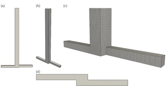
Here, we briefly describe the simulation domain and mesh design used throughout our simu- lations as well as the boundary conditions used and the results from our numerical convergence
FIG. 9. Simulation domain visualized from (a) front view, (b) perspective view, (c) perspective view focused on the junction with outlined grid cells, and (d) bottom view. Grid cells have been purposefully coarsened by a factor of four in each direction for visualization purposes. High resolution simulations were performed with approximately two million grid cells with inlets of length 4L and an outlet of length 15L, where the outlet channel cross section isLbyL. Cell lengths were graded toward the junction by factors of five and ten in the inlets and outlet, respectively.
test. Several representative views of the numerical simulation domain and mesh are presented in Fig.9. All simulations were performed with approximately two million grid cells with inlets of length 4L and an outlet of length 15L, where the outlet channel cross section is L byL. At the
FIG. 10. Convergence test results show the oscillating velocity componentuzat (−0.2, 2, 0) for the St≈ 3.0 state at Re=250. The estimated Strouhal numbers are 3.47 with 1.0×10⁵ cells, 3.00 with 2.5×10⁵ cells, 3.04 with 5.0×10⁵cells, 3.14 with 1.0×10⁶cells, and 3.18 with 2.0×10⁶cells. The relative error in the Strouhal number prediction with 2.0×10⁶cells is less than 1.3%. Note that a third oscillating state with St≈3.0 was identified numerically at higher Reynolds numbers, although it was not found experimentally due to sensitivity to the initial conditions. However, to ensure convergence of all the numerical results, we perform our convergence test on that state since it corresponded to the highest Reynolds number.
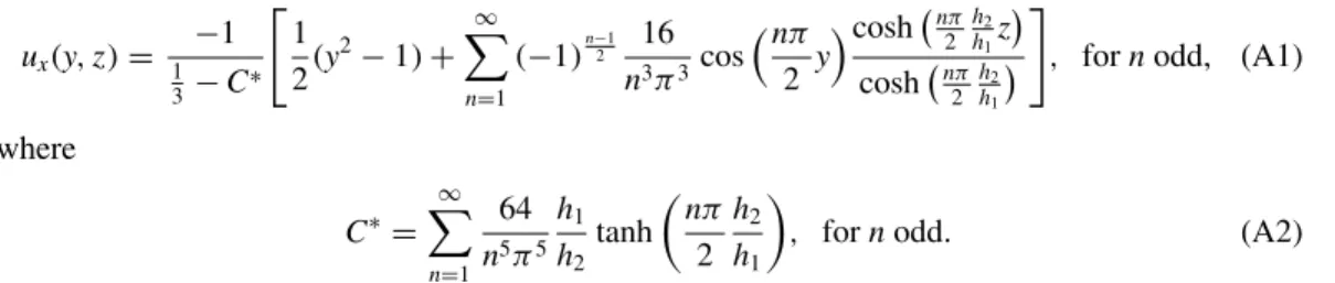
inlets to our system, we specify the well-known fully developed velocity profile for a rectangular duct. With the coordinates defining the cross-section of a square channel given by y,z∈[−1,1]
and nondimensionalized byh1andh2, respectively, the fully developed axial velocity profile along a rectangular channel is given by [39,40]
ux(y,z)= −1
1 3−C∗
1
2(y2−1)+∞
n=1
(−1)n−12 16 n3π3cos
nπ 2 y
cosh n2πhh2
1z cosh n2πhh2
1
, fornodd, (A1) where
C∗= ∞ n=1
64 n5π5
h1 h2tanh
nπ 2
h2 h1
, fornodd. (A2)
Here, the axial velocity profile is nondimensionalized by the average axial flow speed. To set the Reynolds number, we scale the magnitude of this inlet velocity profile and adjust the kinematic viscosity in the solver.
A numerical convergence study was also performed to ensure that the flows were fully resolved.
The results of this study are presented in Fig.10. For the one million and two million grid cell cases, relative difference between the two peak velocities is less than 5%. The convergence study was performed at the highest Reynolds number used in this study of Re=250. At this Reynolds number, a third oscillating flow state appears with St≈3.0. However, we did not include this state in the main text because a sensitivity to initial conditions prevented us from identifying it experimentally.
Nevertheless, since this corresponds to the highest Reynolds number from our study, we selected it for the numerical convergence study.
APPENDIX B: FLOW TRANSITIONS
Here, we present numerical results demonstrating the transient fluid dynamics as the steady-state flow transitions to the different oscillating states. Point particle tracers are generated near the origin
FIG. 11. Growth of the pulsative instability in the steady-state solution at Re=100 as the flow transitions to the pulsating St≈0.5 state. Fluid particles originating nearx=(0,0,0) are visualized over timet. Because the perturbation grows slowly, att=60, the flow is still visually steady. However, with increasing t, the pulsative instability develops upstream and propagates downstream in the outlet channel. Att=140, the flow has approximately transitioned fully to the pulsatile St≈0.5 state.
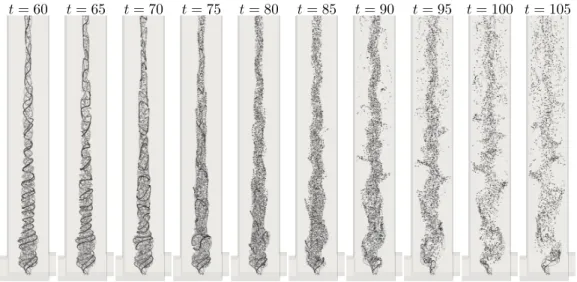
FIG. 12. Growth of the helical instability in the steady-state solution at Re=180 as the flow transitions to the helically oscillating St≈1.75 state. Fluid particles originating nearx=(0,0,0) are visualized over time t. Because the perturbation grows slowly, att=60, the flow is still visually steady. However, with increasingt, the helical instability develops downstream around the third vortex breakdown region and propagates upstream in the outlet channel. Att=105, the flow has approximately transitioned fully to the helically oscillating St≈1.75 state.
x=(0,0,0) and integrated forward in time as the flow evolves. Results demonstrating the transition from the steady state to the pulsating St≈0.5 state are shown in Fig.11, and results showing the transition from the steady state to the helically oscillating St≈1.75 state are shown in Fig.12. For the pulsating St≈0.5 state, the oscillation begins to develop near the first vortex breakdown region in within the junction and propagates downstream as it grows, whereas for the helically oscillating St≈1.75 state, the oscillation begins to develop downstream near the third vortex breakdown region and propagates upstream into the junction as it grows. For each case, the oscillation grows slowly at first so that even att=60 the flows are still apparently steady visually. This is why time begins at t =60 in both figures.
[1] T. B. Benjamin, Theory of the vortex breakdown phenomenon,J. Fluid Mech.14,593(1962).
[2] S. Leibovich, The structure of vortex breakdown,Annu. Rev. Fluid Mech.10,221(1978).
[3] O. Lucca-Negro and T. O’doherty, Vortex breakdown: A review,Prog. Energy Combust. Sci.27,431 (2001).
[4] D. J. C. Dennis, C. Seraudie, and R. J. Poole, Controlling vortex breakdown in swirling pipe flows:
Experiments and simulations,Phys. Fluids26,053602(2014).
[5] S. Pasche, F. Gallaire, M. Dreyer, and M. Farhat, Obstacle-induced spiral vortex breakdown,Exp. Fluids 55,1784(2014).
[6] M. R. Ruith, P. Chen, E. Meiburg, and T. Maxworthy, Three-dimensional vortex breakdown in swirling jets and wakes: Direct numerical simulation,J. Fluid Mech.486,331(2003).
[7] F. Gallaire, M. Ruith, E. Meiburg, J. M. Chomaz, and P. Huerre, Spiral vortex breakdown as a global mode,J. Fluid Mech.549,71(2006).
[8] U. A. Qadri, D. Mistry, and M. P. Juniper, Structural sensitivity of spiral vortex breakdown,J. Fluid Mech.
720,558(2013).
[9] R. Rotunno, The fluid dynamics of tornadoes,Annu. Rev. Fluid Mech.45,59(2013).
[10] R. Davies-Jones, A review of supercell and tornado dynamics,Atmospheric Res.158,274(2015).
[11] N. Syred, A review of oscillation mechanisms and the role of the precessing vortex core (PVC) in swirl combustion systems,Prog. Energy Combust. Sci.32,93(2006).
[12] Y. Huang and V. Yang, Dynamics and stability of lean-premixed swirl-stabilized combustion, Prog.
Energy Combust. Sci.35,293(2009).
[13] C. O. U. Umeh, Z. Rusak, and E. Gutmark, Vortex breakdown in a swirl-stabilized combustor,J. Propul.
Power28,1037(2012).
[14] A. M. Mitchell and J. Délery, Research into vortex breakdown control,Prog. Aerosp. Sci.37,385(2001).
[15] I. Gursul, Z. Wang, and E. Vardaki, Review of flow control mechanisms of leading-edge vortices,Prog.
Aerosp. Sci.43,246(2007).
[16] D. Vigolo, S. Radl, and H. A. Stone, Unexpected trapping of particles at a T junction,Proc. Natl. Acad.
Sci. USA111,4770(2014).
[17] J. T. Ault, A. Fani, K. K. Chen, S. Shin, F. Gallaire, and H. A. Stone, Vortex-Breakdown-Induced Particle Capture in Branching Junctions,Phys. Rev. Lett.117,084501(2016).
[18] S. Shin, J. T. Ault, and H. A. Stone, Flow-driven rapid vesicle fusion via vortex trapping,Langmuir31, 7178(2015).
[19] S. T. Chan, S. J. Haward, and A. Q. Shen, Microscopic investigation of vortex breakdown in a dividing T-junction flow,Phys. Rev. Fluids3,072201(2018).
[20] D. Oettinger, J. T. Ault, H. A. Stone, and G. Haller, Invisible Anchors Trap Particles in Branching Junctions,Phys. Rev. Lett.121,054502(2018).
[21] D. Stoecklein and D. Di Carlo, Nonlinear microfluidics,Anal. Chem.91,296(2018).
[22] J. M. Lopez and F. Marques, Rapidly rotating precessing cylinder flows: Forced triadic resonances, J. Fluid Mech.839,239(2018).
[23] M. A. Ansari, K. Y. Kim, K. Anwar, and S. M. Kim, Vortex micro T-mixer with non-aligned inputs, Chem. Eng. J.181,846(2012).
[24] C. A. Cortes-Quiroz, A. Azarbadegan, and M. Zangeneh, Effect of channel aspect ratio of 3D T-mixer on flow patterns and convective mixing for a wide range of reynolds number,Sens. Actuators B Chem.239, 1153(2017).
[25] C. Hnatovsky, R. S. Taylor, E. Simova, P. P. Rajeev, D. M. Rayner, V. R. Bhardwaj, and P. B. Corkum, Fabrication of microchannels in glass using focused femtosecond laser radiation and selective chemical etching,Appl. Phys. A84,47(2006).
[26] N. Burshtein, S. T. Chan, K. Toda-Peters, A. Q. Shen, and S. J. Haward, 3D-printed glass microfluidics for fluid dynamics and rheology,Curr. Opin. Colloid Interface Sci.43,1(2019).
[27] M. P. Escudier and J. Keller, Recirculation in swirling flow—A manifestation of vortex breakdown,AIAA J.23,111(1985).
[28] M. P. Escudier, A. K. Nickson, and R. J. Poole, Influence of outlet geometry on strongly swirling turbulent flow through a circular tube,Phys. Fluids18,125103(2006).
[29] S. T. Wereley and C. D. Meinhart, Recent advances in microparticle image velocimetry,Annu. Rev. Fluid Mech.42,557(2010).
[30] C. D. Meinhart, S. T. Wereley, and M. H. B. Gray, Volume illumination for two-dimensional particle image velocimetry,Meas. Sci. Technol.11,809(2000).
[31] A. J. Jerri, The Shannon sampling theorem—Its various extensions and applications: A tutorial review, Proc. IEEE65,1565(1977).
[32] H. G. Weller, G. Tabor, H. Jasak, and C. Fureby, A tensorial approach to computational continuum mechanics using object-oriented techniques,Comput. Phys.12,620(1998).
[33] See Supplemental Material at http://link.aps.org/supplemental/10.1103/PhysRevFluids.4.084701 for SIvideo1 shows dye visualization results of the vortex T-mixer flow for Re= {20,40,60,80,100, 120,140,160,180}, which correspond to Fig. 2(a) and SIvideo2 shows animations of the transient simulation results, which correspond to Figs.4(c)and5(c).
[34] J. Jeong and F. Hussain, On the identification of a vortex,J. Fluid Mech.285,69(1995).
[35] P. Chakraborty, S. Balachandar, and R. J. Adrian, On the relationships between local vortex identification schemes,J. Fluid Mech.535,189(2005).
[36] J. M. Lopez, Axisymmetric vortex breakdown part 1: Confined swirling flow,J. Fluid Mech.221,533 (1990).
[37] G. L. Brown and J. M. Lopez, Axisymmetric vortex breakdown part 2: Physical mechanisms,J. Fluid Mech.221,553(1990).
[38] J. M. Lopez and A. D. Perry, Axisymmetric vortex breakdown part 3: Onset of periodic flow and chaotic advection,J. Fluid Mech.234,449(1992).
[39] J. T. Ault, S. Shin, and H. A. Stone, Characterization of surface-solute interactions by diffusio-osmosis, Soft matter15,1582(2019).
[40] F. M. White and I. Corfield,Viscous Fluid Flow(McGraw-Hill, New York, 2006), Vol. 3.