Decomposing Gender Equality along the Wage Distribution in Vietnam during the Period 2002 14

Decomposing Gender Equality along the Wage

Distribution in Vietnam during the Period 2002 14

著者（英） Tien Manh Vu, Hiroyuki Yamada journal or

publication title

AGI Working Paper Series

volume 2017‑04

page range 1‑36

year 2017‑03

URL http://id.nii.ac.jp/1270/00000124/

Decomposing Gender Equality along the Wage Distribution in Vietnam during the Period 2002–14

Tien Manh Vu

Asian Growth Research Institute and Osaka University Hiroyuki Yamada

Faculty of Economics, Keio University Working Paper Series Vol. 2017-04

March 2017

The views expressed in this publication are those of the author(s) and do not necessarily reflect those of the Institute.

No part of this article may be used reproduced in any manner whatsoever without written permission except in the case of brief quotations embodied in articles and reviews. For information, please write to the Institute.

Asian Growth Research Institute

Decomposing Gender Equality along the Wage Distribution in Vietnam during the Period 2002–14

Tien Manh Vu ¹

Asian Growth Research Institute and Osaka University Hiroyuki Yamada

Faculty of Economics, Keio University

Abstract In this paper, we decompose the gender wage gap along the wage distribution in Vietnam during the period 2002–14 and search for the presence of a glass ceiling/sticky floor in wages using the method proposed by Chernozhukov, Fernandez-Val, and Melly (2013). We focus on the formal sector and further divide the sample by educational level, age profile, occupational type, and industry. We find evidence for a total gender wage gap with the price of skills (the price gap) being the main contributor. There are also findings of increases and decreases in equality along the gender wage gap distribution and the formation of a sticky floor and a glass ceiling in 2014 in some of the data.

Key words — gender wage gap, inequality, wage distribution, Vietnam JEL — J31, J71, J16, J21

1

Corresponding author. Contact: 11–4 Otemachi, Kokura-kita, Kitakyushu, Fukuoka 803–0814, JAPAN

Tel.: +81–93–583–6202, Fax: +81–93–583–6576. E–mail: [email protected]

1. INTRODUCTION

Economic growth has generally led to better employment opportunities for Vietnamese women. During the period 2002–14, Vietnam experienced average annual GDP growth in excess of 5%. At the same time, and as shown in Figure 1, there was a sharp increase in the number of private firms replacing the collapse of state-owned enterprises, which once were the most important employers in the economy. These changes, together with Vietnam’s accession to the World Trade Organization in 2007, has led to fierce competition between firms for labor and more formal paid job offers. Vietnam’s low total fertility rate (currently less than 1.95 children per female) and improved levels of education have also provided time and opportunity for Vietnamese women to participate in the labor force and to take up these new job offers. This is evidenced in a female labor participation rate of 73% in 2014 compared with 82% for men (UNDP, 2015), and the ratio of women to men in almost all industries increasing over time, as shown in Figure 2.

[INSERT FIGURES 1 AND 2 HERE]

However, it is not known whether labor market discrimination against women has declined or become more severe along the wage distribution during this period of strong growth and improved employment opportunities. In an increasingly competitive market, firms must minimize business costs or fail. In that sense, any discrimination against gender based on the price of skills (such as education and experience) should raise firm costs. Therefore, gender- based discrimination should decline or even disappear alongside the level of competitiveness.

However, gender wage equality may also vary along the wage distribution, and there is

evidence that the general wage equality has both improved and worsened at various points

during the period 2002–14 (ILO, 2015).

In terms of empirical evidence, Sakellariou and Fang (2014) observed a decrease in private sector wage inequality in Vietnamese households owing to the increase in the minimum wage between 1998 and 2008. Unfortunately, it is unknown whether the gender wage gap in Vietnam persisted. The demonstrated presence of a son preference (Vu, 2014) and the dominance of Confucianism in the country could also be an impediment to decreasing, and could perhaps even be increasing, the gender wage gap. Other forms of derived discrimination are so-called sticky floors and glass ceilings. These kinds of gender discrimination tend to remain severe in either the right- or left-hand tail of the income distribution, such that women are hindered in gaining access to better (and higher paid) positions or are kept in low paid positions. Thus, detecting and tracking the sticky floor and glass ceiling, especially in certain industries and job types, helps to provide valuable labor market policy implications.

Therefore, the purpose of this study is to decompose the gender gap along the wage distribution in Vietnam during the period 2002–14 and to search for the presence of any glass ceiling/sticky floor in women’s wages. We apply a method developed by Chernozhukov, Fernandez-Val, and Melly (2013) to decompose the distribution of the gap into three components; namely, coefficients, characteristics, and residuals. We then compare the distribution of coefficient components across four waves of the Vietnamese household survey for every four-year interval between 2002 and 2014. We select individuals aged from 15 to 55 years of age with only one job and who are not students, self-employed, working for other households, or government officers. Apart from this selected sample, we further divide the data according to educational level, age profile, occupational type, and the two main industries (manufacturing and services) that absorb most paid workers.

Our analysis provides updated insights into the gender wage gap in Vietnam along the wage

distribution and is among a limited number of studies considering the heterogeneity in wages

found among highly educated professionals, occupational types, and industries. We find that

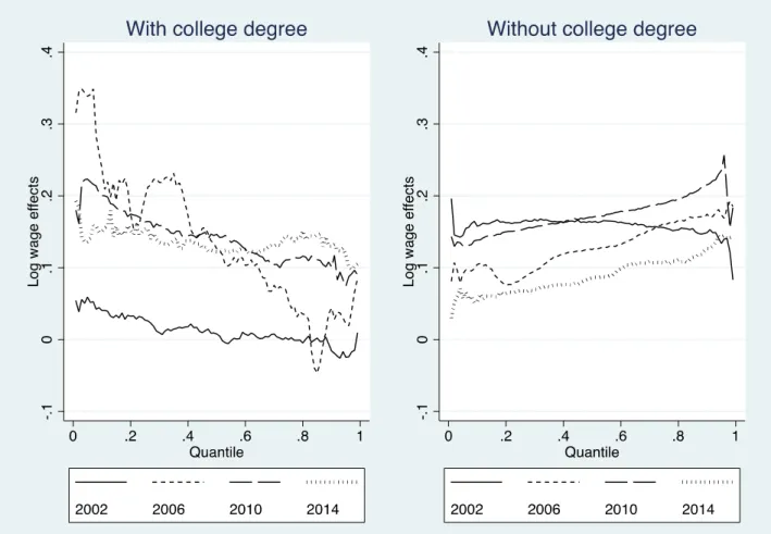
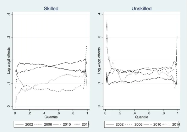
the total gender wage gap (“total gap” hereafter) still exists and that the price of skills (“price gap” hereafter) is the main contributor. We also find evidence of a rise and fall in gender equality along the wage gap distribution, with the total gap gradually becoming greater toward the right (upper) tail of the distribution. There is also an indication of a sticky floor in the total gap in 2014. However, both the total gap and the price gap tend to become narrower in most wage percentiles. Also, we observed rise and fall in equality in the subsamples of workers over time. The price gap is persistent among unskilled (manual) workers but constant along the wage distribution of college graduates. The distribution of the price gap among non-college-educated workers is also increasing, and there is a glass ceiling in the right tail of the distribution in 2014.

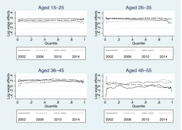
Nevertheless, we find that the price gap has generally fallen in the 15–35-year age thresholds, among skilled workers, and in the manufacturing sector, and is statistically insignificant in the 46–55-year age thresholds and in the service sector.

The remainder of the paper is organized as follows. Section 2 reviews the general literature on the gender wage gap and studies specifically concerning Vietnam. Section 3 details the data used, and Section 4 describes the method. Section 5 discusses the results. Section 6 provides a conclusion.

2. RELATED LITERATURE

Although gender discrimination in wages is closely related to the first target of Goal 5 to

obtain sustainable development recently set by the United Nations, the topic has attracted

significant interest in many countries in the past. Extensive studies on the gender wage gap can

be readily found in the literature, together with the methodological advances in estimation and

decomposition methods necessary to investigate more complicated forms of discrimination

over time. There are various methods available for decomposing the gender wage gap. However,

all of them attempt to identify four desirable decomposed components. The first is the

difference in the price of observable skills. The second is the difference in the return to

unobservable characteristics. The third is the difference in the distribution of observable skills.

The fourth and final component is the difference in the distribution of unobservable characteristics. However, to the best of our knowledge, there is no perfect measure for obtaining these four desired components.

In this regard, Fortin, Lemieux, and Firpo (2011) classified the major decomposition methods into: (a) mean decomposition, such as that employed by Oaxaca (1973) and Blinder (1973), and (b) beyond the mean using variance decomposition, including residual imputation as in Juhn, Murphy, and Pierce (1993), quantile regression such as Machado and Mata (2005), inverse propensity reweighting as in DiNardo, Fortin, and Lemieux (1996), the estimation of conditional distribution, and recentered influence function (RIF) regression (Firpo, Fortin, &

Lemieux, 2009). Each method has both advantages and disadvantages, with most of the mean decomposition methods enabling detailed decomposition, while this is more limited in the approaches in (b) (with the exception of RIF regression). However, the latter group of methods do facilitate analysis of change in the wage distribution, rather than just the mean. The results obtained from decomposing the gender wage gap strongly depend on the country context, when the survey was undertaken, and the selected sample. For this reason, Katz and Autor (1999) recommend that researchers should cautiously examine the robustness of their results in relation to their selection of data source, samples, and method.

In general, the gender wage gap becomes more complex along the wage distribution and

with the level of development, in both developed and developing countries. Examining 26

European countries using 2007 data, Christofides, Polycarpou, and Vrachimis (2013) show that

the size of the gender wage gap differs significantly across countries and that wage

discrimination can appear in either the right or the left tail of the wage distribution. However,

Schober, and Winter-Ebmer (2011) find no causal effect of gender wage equality on economic

growth in their meta-regression of 54 countries during the period 1975–94. The type of

discrimination can also be more complicated than just the paid observable skills. Chzhen and Mumford (2011) suggest a connection between job position, such as high-skilled, white-collar, and managerial posts, and a glass ceiling for full-time workers in Britain in 2005.

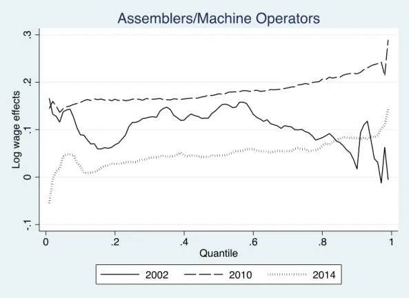
In other work, Albrecht, Björklund, and Vroman (2003) identify a glass ceiling in Sweden in 1998 in the residuals (unknown factors), instead of in the differences in characteristics, sector, industry, and occupation. Similarly, Fang and Sakellariou (2015) reveal the formation of a glass ceiling in six Latin American countries, whereas sticky floor and mixed results are common in six Asian countries. Comparing the 1980s and 1990s, Autor, Katz, and Kearney (2006) suggest that the rapid employment growth in either of the two tails of the skill distribution in the US could be the source for the “polarization” of the wage structure. Coincidentally, we also observe a sharp increase in the proportion of women to men in paid jobs among college graduates and assemblers/machine operators, as shown in Figure 2.

Previous studies on wage equality in Vietnam suggest some gaps in the research. Using the method suggested by Juhn et al. (1991) to analyze two household data sets for Vietnam in 1992–

93 and 1997–98, Liu (2004) identifies that the large positive gap effect overcomes the observed skill and price effects and suggests that Confucianism exerts an influence on the gender wage gap in Vietnam. In other work, Pham and Reilly (2007) find the average gender wage gap decreases during the period 1993–2002 using quantile regressions. They also suggest that there is no “glass ceiling”, at least in two of the survey years examined. However, by the mid- and late- 2000s, the private sector began to dominate employment in Vietnam, and as mentioned, the Vietnamese labor market became more competitive with a larger proportion of female workers in paid employment. Therefore, whether and to what extent the gender wage gap identified in Pham and Reilly (2007) in the early 2000s still exists remains to be investigated.

Later, Sakellariou and Fang (2014) reveal evidence of a more equal gender wage distribution

in the Vietnamese private sector using 1998 and 2008 household surveys. This inspires us to

identify whether the spillover effect that Sakellariou and Fang (2014) identify from the private sector applies between 2002 and 2014. In addition, we also note that 2008 may be a year with unstable economic indicators. According to the International Financial Statistics (IFS) data provided by the International Monetary Fund (IMF), Vietnam experienced high consumer price inflation (CPI) in April–May (21–25%) and August–September (28%). Unfortunately, this was also when the General Statistics Office (GSO) of Vietnam conducted its household survey, and the wage figures gathered may capture noise associated with the short-lived inflationary crisis.

Lastly, Fukase (2014) evaluate the wage premium for workers in foreign firms in Vietnam. The results indicate that the foreign sector absorbed more women and paid a larger wage premium for less-educated women during the period 2002–04. However, there remains a question about any spillover effect from the economy-dominating private sector and whether this has persisted over time.

In terms of background, we should point out that the Vietnamese government raised the minimum wage almost every year between 2004 and 2014. More specifically, the government raised the minimum wage per month for all firms to 290,000, 350,000, 450,000, 830,000, and 1,050,000 Vietnamese dong (VND) in January 2005 (Decree 203/2004/ND-CP), October 2005 (Decree 118/2005/ND-CP), October 2006 (Decree 94/2006/ND-CP), May 2011 (Decree 22/2011/ND-CP), and May 2012 (Decree 31/2012/ND-CP), respectively

. However, a different minimum wage now applies for different regions and in the public and private sectors.

In March 2006, the minimum wage was 870,000 VND for foreign firms in all regions (Decree 03/2006/ND-CP), but from 2008, the minimum wage was set by region. For instance, for foreign firms in Regions 1/2/3/4, the minimum wages were 1.20/1.08/0.95/0.92 million

2

Sakellariou & Fang (2014) conclude that the real minimum wage in Vietnam in 2006 was 1.6 times higher than

that in 2002.

VND in January 2009 (Decree 111/2008/ND-CP), 1.34/1.19/1.04/1.00 million VND from January 2010 (Decree 98/2009/ND-CP), and 1.55/1.35/1.17/1.10 million from January 2011 (Decree 107/2010/ND-CP), respectively. From 2012, the minimum wage varied by region only and was the same for both foreign and domestic firms, with a minimum wage of 2.35/2.10/1.8/1.65 million VND set by Decree 103/2012/ND-CP for Regions 1 to 4 from January 2013 and 2.70/2.40/2.10/1.90 million VND in January 2014 by Decree 182/2013/ND- CP. The reasons for these dissimilar regional settings could be differences in living standards and regional CPI.

The complication of minimum wage settings and the timing of changes is a challenge to any research on impact evaluation, including whether the minimum wage is a causal factor in improving gender wage equality along the wage distribution. A minimum wage may assist women to obtain a better salary and may result in greater wage equality because women are more likely placed in lower-paid jobs. However, changes in labor market equilibriums, such as jobs lost because of the minimum wage, and changes in the pace of wages for each gender along the salary ladder, will make this argument weaker. Another complexity is that changes in the minimum wage may apply to all workers, not just those receiving less than the current minimum wage. This motivates us to perform two tests to confirm whether the minimum wage leads to greater wage equality. The first is whether the residuals contribute significantly to the gender wage gap. The second is whether the price gap declines over time among unskilled positions, which are most likely low-paid jobs, especially among those in the left (lower) tail of the wage distribution.

3. DATA

For our analysis, we use Vietnam household living standard surveys. The GSO conducted

surveys on a 2-year interval using a two-stage stratified sampling method for country

representative samples. The design of the surveys follows the Living Standards Measurement

Study by the World Bank. We include four-year interval waves for our analysis, thereby including the surveys conducted in 2002 (29,532 households), 2006 (9,189 households), 2010 (46,995 households), and 2014 (9,399 households). The surveys contain information on wages, age and gender, work hours per day, work days per month, work months per year, and occupational type and industry for all those with some income in the 12-month period prior to the time of the survey.

We attempt to focus on formal employment and to select only those individuals closest to the definition of the International Labor Organization (ILO) for employment (ILO, 2013).

Accordingly, we select individuals from 15 to 55 years of age who are not students, not self- employed, not working for other households, and not government officers, and who have only one job at a time

. We trim the data by 0.1% at both ends of the income distribution

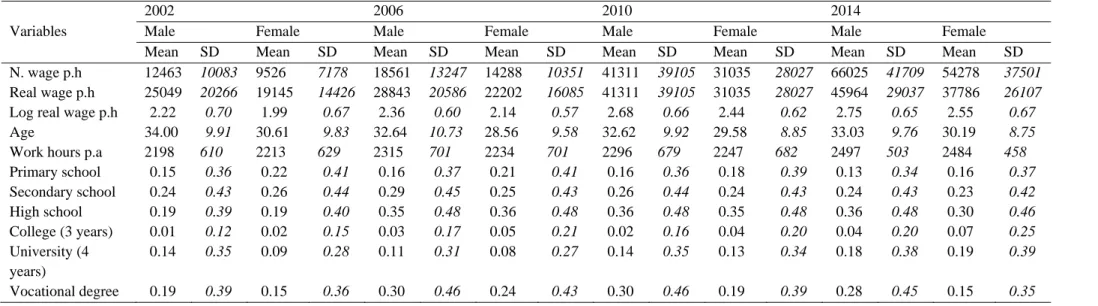
. Table 1 details the sample size and characteristics by gender in each survey wave.

[INSERT TABLE 1 HERE]

As shown in Table 1, men are more likely than women to have a paid job. However, the participation rate of women for any of the selected samples is higher than the corresponding rate for men. In the selected sample, men are about 3–4 years older than women, although their average working hours per year are quite similar (approximately 2,198 hours).

3

The retirement age in Vietnam is 55 years for women and 60 years for men. One outcome is that women are more likely to work part-time or in the informal labor sector after retirement. Meanwhile, those with more two jobs at the same time are more likely employed part-time or in agriculture. Therefore, our sample selection criteria are stricter than those of Pham & Reilly (2007), but this increases the chance of finding an individual of opposite gender but similar in individual characteristics and employment nature.

4

About 75% (90%) of all individuals work more than 2,112 (1,414) hours per year or 40.6 (27.2) hours per week

in 52 working weeks.

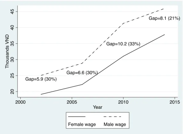
The wage per hour (in logarithms) is calculated using the total income from paid employment, including salary, related cash and goods in kind (comprising holiday bonuses, bonuses, and subsidies), and the total working hours for the last 12 months prior to the survey.

Total working hours is derived from the average working hours per day, average days per month, and average months per year in a 12-month period. We convert the calculated log wage to 2010 base prices. Although there is already evidence of an average gender wage gap of approximately 6,000–10,000 VND per hour (2010 prices), corresponding to a gender wage gap of 21–33.1%, as shown in Figure 3, we decompose the gap using the method described in the next section.

[INSERT FIGURE 3 HERE]

4. ECONOMETRIC METHOD AND SPECIFICATION

We apply the method suggested by Chernozhukov, Fernandez-Val, and Melly (2013) (CFM hereafter)

. This relies on two estimated counterfactual distributions. The first is estimated from the characteristics distribution (the distribution of skills) for the group of men, the median (mean) coefficients (price of skills) from the group of men, and the residual distribution from the group of women. The second is from the characteristics distribution for the group of men, and the conditional distribution of the skills of women

. The two estimated distributions are then used to decompose the total difference into three components: coefficients, characteristics, and residuals (as suggested by Juhn et al., 1993).

5

We use the user-written Stata command, ‘cdeco_jmp’, by Chernozhukov, Fernandez-Val, & Melly. The package is available at https://sites.google.com/site/blaisemelly/computer-programs/inference-on-counterfactual- distributions.

6

The linear quantile regression estimator in Koenker & Bassett (1978) and the rearrangement method in

Chernozhukov, Fernandez-Val, & Galichon (2010) are used to estimate the conditional distribution.

More specifically, the method follows a procedure introduced by Melly (2005). Melly’s (2005) suggestion is to estimate the counterfactual distribution of wages that would hold among women if their distribution of skills was the same as that for men. The quantile of the counterfactual distribution of the wage is then ,

, where is the estimated coefficient of women from a linear quantile regression suggested by Koenker and Bassett (1978) and is a vector of the characteristics of men. Similarly, changes in characteristics (skills) explain the difference between , and , . Next, the distribution of the wage that would hold if the median return to skills for women were the same as among males but the residuals were the same as among females is

, . Changes in the coefficients explain the difference between

, and , . Similarly, the gap between

, and

, is explained by changes in the residuals. The total gender wage gap can be decomposed as

, , ,

,

,

, , , . (1)

Thus, (2) can be simplified to

. (2)

The CFM method has advantages and disadvantages. By using a form of quantile regression to estimate the distribution of the residuals, the method does not have to assume that the

7

See Melly (2005) for details.

residuals are independent of the characteristics (skills). The method is also path independent.

The results of the decomposition are then not influenced by the order in which the various components of the detailed decomposition are calculated. A joint test for the positive gender gap (the constant effect) in all percentiles is possible, which directly helps us to respond to our first research question. Unfortunately, the method is unable to provide detailed decomposition as contributed by each of the covariates.

We set the same specification for all waves. We define skills as the education and age of the individual. We use dummy variables to identify the level of education, comprising 3-year college, 4-year university, senior high school (12 years of general education), junior high school (9 years of general education), and primary school (5 years of general education) graduates

. We did not use the projected experience calculated from age minus years of schooling minus seven years

. Instead, we use age and squared age as the proximate values. Unfortunately, we do not have information on tenure or length of job, and we acknowledge this limitation. As our focus is the price of skills, we assume that other possible factors, such as the differences in occupational type and industry, reside in the residuals. We set a bootstrap of 100 repetitions in our estimation. We do not include 2002 in our analysis by industry because the classification of industries in that survey wave was too simple. In addition, to address the heterogeneity identified by Fortin and Lemieux (2016) and Grund (2015), we divide the selected sample according to highly educated professionals, age profile, occupational types, and industry, and repeat the analysis for additional insights.

8

Later, we define college graduates as anyone with either a 3-year college or 4-year university degree.

9

This is unreasonable because we find that some individuals acquired additional qualifications while working.

Thus, some have negative projected experience. In addition, the available information on experience in the 2006

wave shows that the differences between projected and actual work experience are significant.

We identify sticky floors/glass ceilings using the definition suggested by Arulampalam, Booth, and Bryan (2007). We define a sticky floor/glass ceiling as being present when the top- 10 percentile of the corresponding tail is 2% higher than any percentile in the middle of the distribution. More specifically, a sticky floor (glass ceiling) is only when every 1

–10

(90

– 99

) percentile passes at least 78 tests. The null hypothesis of each test is that the estimated difference in a percentile of the tail is 2% higher than another percentile in the 11

–89

percentile at the 95% level of confidence. Lastly, we decompose the gender wage gap using several alternative methods, including ordinary least squares estimation (OLS), the standard Oaxaca (1973) and Blinder (1973) (OB) approach, the standard JMP approach from Juhn et al.

(1993), and the RIF regression from Firpo et al. (2009) for robustness.

5. RESULTS

5.1. Full sample

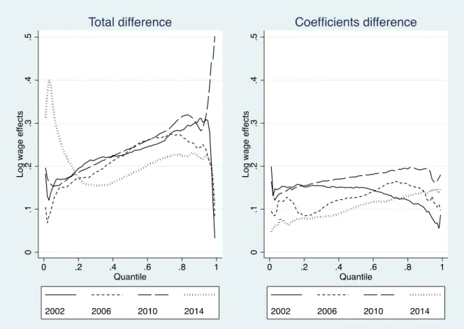
We find three important pieces of evidence concerning the gender wage gap and the price gap in Vietnam. First, the total gap and the price gap remain statistically significant in all waves, as shown in Figure 4 and the test results in column T1 of Table 2. The results are also consistent when we apply the other methods described in Appendix 1. Although more women are in paid work in 2014 than in 2002, wage discrimination persists.

[INSERT FIGURE 4 HERE]

[INSERT TABLEs 2 AND 3 HERE]

Second, the total gap is not constant along the distribution. All tests for a constant quantile effect are rejected (column T2 in Table 2). With the exception of 2014, the total gap tends to increase with the percentile. Moreover, as depicted in Figure 4, a sticky floor formed in 2014.

The test for a sticky floor in column T3 of Table 3 confirms our visual inspection. Nevertheless,

the price gap does not contribute significantly to the sticky floor in the total gap (only about 26% of the floor) in 2014. These results contrast with previous findings in Pham and Reilly (2007). Pham and Reilly (2007) found that the treatment effect was stable along the conditional wage distribution during the period 1993–2002. However, our results are similar to those identified by Duraisamy and Duraisamy (2016) in India during the period 1983–2012. Thus, our results suggest that gender inequality along the wage distribution is becoming more complicated.

Finally, other than a decrease in equality in 2010, we find that the total gap and price gap become smaller over time, as shown in both Figure 4 and Table 2. The price gap likely narrows in the left tail of the price gap distribution over time (see Figure 4). This result demonstrates that the decreasing gender wage gap trend first identified in Pham and Reilly (2007) continues after the period 1993–2002.

Other than this, we find little evidence to support the argument that a change in minimum wage helps to increase gender equality, at least in our selected sample

. Part of the market interventions, that is, the minimum wage settings, are captured in the residuals. From the decomposition of the gender wage gap, we find that the residuals play a very minor role in the total gender gap in 2006 and 2014. We are unable to reject the hypothesis that all the quantile effects of the residuals equal zero, as shown in column T1 of Table 2 (a visual result is in Appendix 2). Other parts of the interventions may reside in the price of skills. As shown in the next subsection, this could be a reasonable candidate for explaining the gender wage gap among

10

We acknowledge that a small proportion of individuals in our selected sample are paid around the minimum

wage. The percentages of those who received less than 120% of the minimum wage in 2002 are just 1.8 and 2.3

for males and 1.4 and 2.1 for females, respectively. The corresponding figures are 1, 1.4, 1.6, and 2.1 in 2006, 1.2,

1.5, 1.4, and 1.7 in 2010, and 1.4, 2.1, 2.5 and 3.5 in 2014. However, if the salaries of those paid above the

minimum wage are calculated based on the minimum wage as a unit, our tests hold.

those who are assemblers or machine operators and not college graduates. However, this argument cannot explain the persistent price gap among unskilled (worker) positions, which are most likely paid closer to the minimum wage.

5.2. Subsamples

After dividing the selected sample into its various subcategories, we observe complex increases and decreases in the price gap. First, we observe a different trend for college and non- college graduates. If we exclude 2010, equality increases over time among non-college graduates, as shown in Figure 5 and Table 3. However, the price gap tends to narrow faster in the left tail of the distribution. As the result, a glass ceiling (price gap) forms in 2014, as the test results show in column T3 of Table 3. Meanwhile, the price gap is more persistent after 2006 among college graduates, as shown in Table 3 and Figure 5. In 2002 and 2006, the hypothesis of all quantile effects being equal to zero fails to be rejected. In contrast, the quantile effects are all significant in 2010 and 2014 (see column T1 in Table 3). In addition, in 2014, we observe a sticky floor in the total gap distribution. Thus, among college graduates, gender wage inequality increases, even though inequality tends to be constant in all percentiles, as shown in column T2 in Table 3.

[INSERT FIGURES 5 AND 6 HERE]

Second, in the decomposition results by age category, we observe similar complexities, as shown in Table 3 and Figure 6. The price gap is significant and is lowest in 2014 for ages 15–

25 and 26–35. In contrast, the price gap for ages 46–55 is minimal. Tests for all quantile effects

being zero are not rejected in any of the selected years. However, the price gap is persistent

among those aged 36–45. In addition, we should note that the age profiles could exhibit

generational change in that the majority of those aged 15–25 (26–35, 36–45) in 2002 turned

27–35 (38–45, 48–55) in 2014. If these were developing constantly in terms of experience with

the same amount of education, the corresponding results in Table 3 should also show a reduction in gender inequality, with the exception of those aged 38–45 in 2014. However, we acknowledge that our results do not properly illustrate the inequality within the wage distribution for each gender separately.

[INSERT TABLE 4 HERE]

[INSERT FIGURES 7, 8 AND 9 HERE]

Finally, we identify a persistent price gap among skilled and unskilled workers. In contrast, we observe only a small price gap for assemblers/machine operators in 2014, as shown in Table 4 and Figures 7 and 8. Meanwhile, Table 4 and Figure 9 indicate an increase in wage equality in both the manufacturing and service sectors. The hypothesis that all quantile effects (the price gap) in 2014 are zero is not rejected.

6. CONCLUSIONS

We decompose the wage inequality along the wage distribution by gender in Vietnam during the period 2002–14. We find evidence of both severer inequality and improving equality. In general, the total gap appears to be persistent, mainly because of gender discrimination in the price of skills. However, the total gap is not constant throughout the distribution and is wider in the right (upper) tail. We identify several different items of evidence for a sticky floor and a glass ceiling for the total gap and price gap in particular years, but there is no consistent trend.

Meanwhile, there is an increase in wage equality over time as the wage gap has tended to narrow

(except in 2010). The price gap has decreased among those aged 15–35, among skilled workers,

and those in the manufacturing sector, and has becomes insignificant among those aged 46–55

and those in the service sector. However, we find little evidence to support the argument that

the decreasing gap is because of the higher (real) minimum wage.

Our findings suggest several policy implications and directions for future research. We first recommend the adding of articles on equal pay and equal opportunity to the Laws of Labor in Vietnam. A glass ceiling in the price gap appears among non-college graduates because the speed of narrowing of the gap is faster in the left (lower) than in the right (upper) tail. Therefore, using enforced laws to break the practice of discrimination against women at a higher level of income is more imperative, although the free market could adjust for this more naturally but over a longer time. Meanwhile, we would suggest that any policy creating competitiveness, especially in the growth of the private sector, would also promote gender equality given that the price gap still contributes most to the gender wage gap. Pressure from rival firms would induce employers to remove any gender discrimination on the price of skills. Finally, when data from future surveys become available, we recommend reexamination of the sticky floor in the total gender wage gap that we found in 2014.

Acknowledgement: This work was supported by JSPS (Japan Society for the Promotion of

Science) KAKENHI Grant Number 15H01950, a project grant from the Asian Growth

Research Institute, and a grant from the MEXT Joint Usage/Research Center at the Institute of

Social and Economic Research, Osaka University.

REFERENCES

Albrecht, J., Björklund, A., & Vroman, S. (2003). Is there a glass ceiling in Sweden? Journal of Labor Economics, 21(1), 145–177.

Arulampalam, W., Booth, A. L., & Bryan, M. L. (2007). Is there a glass ceiling over Europe?

Exploring the gender pay gap across the wage. Industrial and Labor Relations Review, 60(2), 163–186.

Autor, D., Katz, L., & Kearney, M. (2006). The polarization of the U.S. labor market. American Economic Review, 96(2), 189–194.

Blinder, A. S. (1973). Wage discrimination: Reduced form and structural estimates. Journal of Human Resources, 8(4), 436–455.

Chernozhukov, V., Fernandez-Val, I., & Melly, B. (2013). Inference on counterfactual distributions. Econometrica, 81(6), 2205–2268.

Chernozhukov, V., Fernandez-Val, I., & Galichon, A. (2010). Quantile and probability curves without crossing. Econometrica, 78(3), 1093–1125.

Christofides, L. N., Polycarpou, A., & Vrachimis, K. (2013). Gender wage gaps, “sticky floors”

and “glass ceilings” in Europe. Labour Economics, 21, 86–102.

Chzhen, Y., & Mumford, K. (2011). Gender gaps across the earnings distribution for full-time employees in Britain: Allowing for sample selection. Labour Economics, 18(6), 837–844.

DiNardo, B. Y. J., Fortin, N. M., & Lemieux, T. (1996). Labor market institutions and the distribution of wages, 1973–1992: A semiparametric approach. Econometrica, 64(5), 1001–1044.

Duraisamy, M., & Duraisamy, P. (2016). Gender wage gap across the wage distribution in

different segments of the Indian labour market, 1983–2012: Exploring the glass ceiling

or sticky floor phenomenon. Applied Economics, 48(43), 4098–4111.

Fang, Z., & Sakellariou, C. (2015). Glass ceilings versus sticky floors: Evidence from Southeast Asia and an international update. Asian Economic Journal, 29(3), 215–242.

Firpo, S., Fortin, N. M., & Lemieux, T. (2009). Unconditional quantile regressions.

Econometrica, 77(3), 953–973.

Fortin, N., Lemieux, T., & Firpo, S. (2011). Chapter 1 – Decomposition methods in economics.

In Handbook of labor economics (Vol. 4, pp. 1–102, North Holland).

Fortin, N., & Lemieux, T. (2016). Inequality and changes in task prices: Within and between occupation effects. In L. Cappellari, S. W. Polachek, & K. Tatsiramos (Eds.), Inequality:

Causes and consequences (Research in Labor Economics, Vol. 43, pp. 195 – 226, Emerald Group Publishing Limited).

Fukase, E. (2014). Foreign wage premium, gender and education: insights from Vietnam household surveys. The World Economy, 37(6), 834–855.

Grund, C. (2015). Gender pay gaps among highly educated professionals — Compensation components do matter. Labour Economics, 34, 118–126.

International Labour Organization. (ILO). (2013). Resolution I - Resolution concerning statistics of work, employment and labour underutilization.

http://www.ilo.org/wcmsp5/groups/public/---dgreports/---

stat/documents/normativeinstrument/wcms_230304.pdf. Last accessed Jan 2017.

International Labour Organisation. (ILO). (2015). Global Wage Report 2014/15: Wage and Income Inequality. Geneva: ILO.

Juhn, C., Murphy, K. M., & Pierce, B. (1993). Wage inequality and the rise in returns to skill.

Journal of Political Economy, 101(3), 410–442.

Katz, L. F., & Autor, D. H. (1999). Changes in the wage structure and earnings inequality. In

Handbook of labor economics (Vol. 3, pp. 1463–1555, North Holland).

Liu, A. Y. C. (2004). Gender wage gap in Vietnam: 1993 to 1998. Journal of Comparative Economics, 32(3), 586–596.

Melly, B. (2005). Decomposition of differences in distribution using quantile regression.

Labour Economics, 12(4), 577–590.

Koenker, R., & Bassett, G. (1978). Regression quantiles. Econometrica, 46, 33–50.

Oaxaca, R. (1973). Male–female wage differentials in urban labor markets. International Economic Review, 14(3), 693–709.

Pham, T.-H., & Reilly, B. (2007). The gender pay gap in Vietnam, 1993–2002: A quantile regression approach. Journal of Asian Economics, 18(5), 775–808.

Sakellariou, C., & Fang, Z. (2014). The Vietnam reforms, change in wage inequality and the role of the minimum wage. Economics of Transition, 22(2), 313–340.

Schober, T., & Winter-Ebmer, R. (2011). Gender wage inequality and economic growth: Is there really a puzzle?—A comment. World Development, 39(8), 1476–1484.

United Nations Development Programme (UNDP). (2015). UNDP Human Development Report 2015. http://hdr.undp.org/sites/all/themes/hdr_theme/country-notes/VNM.pdf.

Last accessed Jan 2017.

Vu, T. M. (2014). One male offspring preference: Evidence from Vietnam using a split-

population model. Review of Economics of the Household, 12(4), 689–715.

Appendix 1. Comparing gender gap in different methods of estimation

Method Gender wage gap Total difference Difference by coefficients (price)

2002 2006 2010 2014 2002 2006 2010 2014

OLS Marginal effect 0.14 0.124 0.17 0.12

O-B Raw 0.23 0.19 0.22 0.186 58–60% 63–65% 81–77% 73–60%

JMP At Mean 0.23 0.19 0.22 0.20 0.14 0.12 0.17 0.12

RIF At

10

0.17 0.15 0.17 0.20 0.11 0.11 0.12 0.08

25

0.21 0.17 0.19 0.15 0.13 0.11 0.13 0.09

50

0.23 0.22 0.24 0.15 0.13 0.13 0.17 0.08

75

0.28 0.27 0.30 0.25 0.17 0.15 0.23 0.16

90

0.29 0.26 0.30 0.23 0.17 0.15 0.23 0.15

CFM At

10

0.17 0.15 0.16 0.25 0.15 (89%) 0.13 (85%) 0.14 (90%) 0.07 (27%)

25

0.21 0.17 0.19 0.16 0.16 (74%) 0.09 (52%) 0.16 (82%) 0.08 (50%)

50

0.23 0.24 0.24 0.18 0.15 (65%) 0.13 (53%) 0.18 (73%) 0.11 (58%)

75

0.28 0.27 0.30 0.23 0.12 (44%) 0.16 (60%) 0.19 (65%) 0.12 (55%)

90

0.31 0.24 0.29 0.22 0.10 (32%) 0.14 (56%) 0.19 (67%) 0.14 (63%)

Notes: All the estimated coefficients are statistically significant except the 10

percentile in 2014. OLS (Ordinary Least Squares estimation using gender as a dummy)/OB

(Oaxaca–Blinder)/JMP (Juhn, Murphy, and Pierce) /RIF (Recentered Influence Function)/CFM (Chernozhukov, Fernandez-Val, & Melly, 2013) estimations use the same

explanatory variables.

Appendix 2. Gender wage gap contributed by the residuals and year

Figure 1. Share of employees by economic sectors, gender, and year.

Source: Authors’ calculations from the Vietnamese Household Living Standard Survey 2002, 2006, 2010, and 2014.

Notes: SOE: State-owned enterprises. PDE: Private domestic (non-foreign) enterprises. FOE: foreign-owned

(affiliated) enterprises.

Figure 2. Average ratio of employed females to employed males by education, job position, and industry.

Source: Authors’ calculation from the Vietnamese Household Living Standard Survey 2002, 2006, 2010, and

2014.

Figure 3. Mean real wage (2010 prices).

Source: Authors’ calculation from the Vietnamese Household Living Standard Survey 2002, 2006, 2010, and 2014.

Note: Gap unit is VND 1,000.

Figure 4. Total gender gap and decomposed gap by coefficients.

Figure 5. Decomposed gender gap contributed by coefficients by educational achievements.

Figure 6. Decomposed gender gap contributed by coefficients by age profiles.

Figure 7. Price gaps for skilled and unskilled positions.

Figure 8. Price gaps for assemblers and machine operators.

Figure 9. Price gaps for manufacturing and service sectors.

Table 1. Descriptive statistics

2002 2006 2010 2014

Variables Male Female Male Female Male Female Male Female

Mean SD Mean SD Mean SD Mean SD Mean SD Mean SD Mean SD Mean SD N. wage p.h 12463 10083 9526 7178 18561 13247 14288 10351 41311 39105 31035 28027 66025 41709 54278 37501 Real wage p.h 25049 20266 19145 14426 28843 20586 22202 16085 41311 39105 31035 28027 45964 29037 37786 26107 Log real wage p.h 2.22 0.70 1.99 0.67 2.36 0.60 2.14 0.57 2.68 0.66 2.44 0.62 2.75 0.65 2.55 0.67 Age 34.00 9.91 30.61 9.83 32.64 10.73 28.56 9.58 32.62 9.92 29.58 8.85 33.03 9.76 30.19 8.75 Work hours p.a 2198 610 2213 629 2315 701 2234 701 2296 679 2247 682 2497 503 2484 458 Primary school 0.15 0.36 0.22 0.41 0.16 0.37 0.21 0.41 0.16 0.36 0.18 0.39 0.13 0.34 0.16 0.37 Secondary school 0.24 0.43 0.26 0.44 0.29 0.45 0.25 0.43 0.26 0.44 0.24 0.43 0.24 0.43 0.23 0.42 High school 0.19 0.39 0.19 0.40 0.35 0.48 0.36 0.48 0.36 0.48 0.35 0.48 0.36 0.48 0.30 0.46 College (3 years) 0.01 0.12 0.02 0.15 0.03 0.17 0.05 0.21 0.02 0.16 0.04 0.20 0.04 0.20 0.07 0.25 University (4

years)

0.14 0.35 0.09 0.28 0.11 0.31 0.08 0.27 0.14 0.35 0.13 0.34 0.18 0.38 0.19 0.39

Vocational degree 0.19 0.39 0.15 0.36 0.30 0.46 0.24 0.43 0.30 0.46 0.19 0.39 0.28 0.45 0.15 0.35

Table 1. Cont.

2002 2006 2010 2014

Variables Male Female Male Female Male Female Male Female

Mean SD Mean SD Mean SD Mean SD Mean SD Mean SD Mean SD Mean SD Job rank/types

Skilled worker 1 0.07 0.26 0.03 0.18 0.08 0.27 0.05 0.21 0.12 0.32 0.08 0.28 0.14 0.34 0.08 0.27 Skilled worker 2 0.03 0.17 0.04 0.20 0.01 0.08 0.01 0.11 0.01 0.12 0.01 0.10 0.01 0.12 0.01 0.09 Skilled worker 3 0.26 0.44 0.34 0.47 0.24 0.43 0.34 0.47 0.23 0.42 0.26 0.44 0.22 0.41 0.21 0.41 Assemblers 0.14 0.35 0.05 0.22 0.14 0.35 0.05 0.22 0.23 0.42 0.19 0.39 0.23 0.42 0.24 0.43 Unskilled worker 0.26 0.44 0.28 0.45 0.27 0.44 0.29 0.45 0.16 0.36 0.16 0.36 0.15 0.35 0.15 0.35 Industries

Manufacturing 0.41 0.49 0.63 0.48 0.40 0.49 0.62 0.48 0.42 0.49 0.61 0.49 Services

Cat. 1 0.10 0.30 0.07 0.26 0.12 0.33 0.09 0.29 0.12 0.33 0.10 0.30 Cat. 2 0.03 0.18 0.04 0.20 0.03 0.17 0.04 0.18 0.03 0.16 0.03 0.17 Cat. 3 0.00 0.05 0.00 0.04 0.02 0.15 0.02 0.13 0.02 0.14 0.01 0.12 Cat. 4 0.01 0.11 0.02 0.15 0.02 0.13 0.03 0.16 0.02 0.14 0.03 0.17 Cat. 5 0.00 0.00 0.00 0.00 0.00 0.07 0.00 0.06 0.00 0.06 0.00 0.05 Cat. 6 0.00 0.00 0.00 0.00 0.02 0.14 0.01 0.12 0.02 0.14 0.02 0.14 Cat. 7 0.00 0.00 0.00 0.00 0.01 0.11 0.01 0.11 0.02 0.14 0.01 0.11 Selected sample size 2,407 2,044 860 751 5,243 4,448 1,181 1,164 Any employee** 15,841 9,962 3,965 2,558 21,262 14,474 4,418 3,158 Any nonstudent** 32,547 34,743 10,185 10,519 57,229 58,588 10,764 10,883

Notes: Real wage based on 2010 prices using World Bank CPI: http://data.worldbank.org/indicator/FP.CPI.TOTL?end=2015&locations=VN&start=2000). **: individuals are

nonstudents and between 15–55 years of age.

Table 2. Total gender gap and decomposed gaps by coefficients and residuals

Percentile 10

25

50

75

90

T1 T2 T3

Year Total gap

2002 0.17 (0.03) 89.01 0.21 (0.02) 74.28 0.23 (0.02) 65.24 0.28 (0.03) 43.97 0.31 (0.04) 32.45 R A-r 2006 0.15 (0.04) 85.28 0.17 (0.03) 52.10 0.24 (0.03) 53.22 0.27 (0.04) 60.12 0.24 (0.06) 56.45 R A-r 2010 0.16 (0.02) 89.67 0.19 (0.01) 82.10 0.24 (0.01) 72.62 0.30 (0.02) 65.15 0.29 (0.03) 67.48 R A-r 2014 0.25 (0.07) 26.55 0.16 (0.03) 50.23 0.18 (0.02) 57.90 0.23 (0.03) 54.83 0.22 (0.04) 63.13 R A-r S Year Decomposed gap by coefficients

2002 0.15 (0.03) 0.16 (0.03) 0.15 (0.02) 0.12 (0.03) 0.10 (0.04) R A-a 2006 0.13 (0.03) 0.09 (0.03) 0.13 (0.03) 0.16 (0.03) 0.14 (0.05) R A-r

2010 0.14 (0.01) 0.16 (0.01) 0.18 (0.01) 0.19 (0.01) 0.19 (0.02) R A-r

2014 0.07 (0.04) 0.08 (0.03) 0.11 (0.03) 0.12 (0.03) 0.14 (0.04) R A-r Year Decomposed gap by residuals

2002 –0.05 (0.03) –0.03 (0.02) –0.02 (0.01) 0.05 (0.02) 0.09 (0.04) R A-r

2006 –0.02 (0.05) 0.02 (0.03) 0.02 (0.02) 0.00 (0.03) 0.00 (0.04) A A-a

2010 –0.03 (0.02) –0.01 (0.01) 0.00 (0.01) 0.03 (0.01) 0.02 (0.02) R A-r

2014 0.07 (0.06) 0.01 (0.02) 0.00 (0.02) 0.04 (0.02) 0.02 (0.03) A A-a Notes:

Listed values are for the i

percentile. However, we estimated and conducted the tests of hypotheses for all percentiles and for each percentile from 1

to 99

. Pointwise standard errors in parentheses are obtained from an empirical bootstrap of 100 repetitions. We employ Cramer–von Mises–Smirnov (main reference) and Kolmogorov–

Smirnov statistics to decide the test results.

T1: Test results for H0: No effect, QE(tau)=0 for all taus from 1–99. If H0 is rejected (10% level), then “R”. If H0 is not rejected, then “A”. This test is stronger than the absence of any mean effect.

Figures in italics are percentages of the gender wage gap contributed by coefficients.

T2: Test results for two hypotheses in the following order.

H0: Stochastic dominance: QE(tau)>0 for all taus from 1 to 99. If H0 is not rejected, then “A”, otherwise “R”.

H0: Constant effect: QE(tau)=QE(0.5) (10% level). If H0 is not rejected, then “a”, otherwise “r”.

T3: H0: Sticky floor /H0: Glass ceiling. S (G) is denoted only if all 1

–10

(90

–99

) percentiles passed at least 78 tests that the estimated difference of the percentile is 2%

higher than those of 11

–89

percentiles (5% level).

Table 3. Decomposed gender gap contributed by coefficients in subsamples

Year 10

25

50

75

90

T1 T2 T3 T4

College degree

2002 0.04 (0.10) 0.03 (0.09) 0.01 (0.08) 0.00 (0.08) –0.02 (0.08) A A-a 2006 0.24 (0.15) 0.20 (0.14) 0.13 (0.11) 0.05 (0.11) 0.04 (0.12) A A-a 2010 0.20 (0.05) 0.16 (0.05) 0.15 (0.04) 0.11 (0.05) 0.10 (0.04) R A-a

2014 0.15 (0.10) 0.15 (0.08) 0.12 (0.06) 0.14 (0.05) 0.13 (0.06) R A-a S

No college degree

2002 0.16 (0.03) 0.16 (0.03) 0.16 (0.02) 0.16 (0.02) 0.15 (0.03) R A-a 2006 0.10 (0.04) 0.08 (0.04) 0.13 (0.03) 0.16 (0.03) 0.17 (0.04) R A-r

2010 0.14 (0.01) 0.15 (0.01) 0.17 (0.01) 0.19 (0.01) 0.22 (0.01) R A-r G 2014 0.05 (0.04) 0.07 (0.03) 0.09 (0.03) 0.11 (0.03) 0.13 (0.03) R A-r G

Age 15–25

2002 0.16 (0.05) 0.17 (0.04) 0.17 (0.04) 0.18 (0.03) 0.16 (0.04) R A-a 2006 0.10 (0.05) 0.06 (0.04) 0.11 (0.04) 0.09 (0.05) 0.10 (0.06) R A-a

2010 0.09 (0.03) 0.10 (0.02) 0.11 (0.02) 0.12 (0.02) 0.16 (0.03) R A-a G 2014 0.07 (0.08) 0.05 (0.07) 0.04 (0.06) 0.04 (0.05) 0.06 (0.08) A A-a

Age 26–35

2002 0.17 (0.04) 0.16 (0.04) 0.15 (0.04) 0.13 (0.04) 0.12 (0.05) R A-a 2006 0.20 (0.08) 0.20 (0.06) 0.18 (0.06) 0.21 (0.07) 0.18 (0.12) R A-a 2010 0.19 (0.02) 0.20 (0.02) 0.20 (0.02) 0.19 (0.02) 0.17 (0.03) R A-a 2014 0.06 (0.05) 0.08 (0.04) 0.11 (0.03) 0.10 (0.04) 0.08 (0.04) R A-a

Age 36–45

2002 0.22 (0.05) 0.22 (0.05) 0.24 (0.04) 0.18 (0.05) 0.18 (0.05) R A-a 2006 0.16 (0.15) 0.17 (0.10) 0.16 (0.11) 0.18 (0.09) 0.15 (0.11) A A-a 2010 0.23 (0.03) 0.24 (0.03) 0.27 (0.03) 0.25 (0.03) 0.20 (0.04) R A-a 2014 0.10 (0.07) 0.13 (0.06) 0.16 (0.06) 0.20 (0.06) 0.22 (0.10) R A-a

Age 46–55

2002 –0.08 (0.10) –0.01 (0.08) –0.02 (0.07) 0.01 (0.07) –0.05 (0.09) A A-a 2006 0.10 (0.13) 0.04 (0.12) 0.15 (0.11) 0.15 (0.14) 0.11 (0.18) A A-a

2010 0.11 (0.05) 0.08 (0.05) 0.06 (0.05) –0.02 (0.05) –0.06 (0.08) A A-a S 2014 0.13 (0.19) 0.10 (0.12) 0.17 (0.10) 0.17 (0.09) 0.26 (0.12) A A-a

Notes are the same as for Table 2.

T4 shows the conclusion on the distribution of total gap with H0: Sticky floor /H0: Glass ceiling. S (G) is denoted only if all 1

– 10

(90

– 99

) percentiles passed at least 78

tests that the estimated difference of the percentile is 2% higher than those of 11

– 89

percentiles (5% level).

Table 4. Decomposed gender wage gap by coefficients in subsamples

Year 10

25

50

75

90

T1 T2 T3 T4

Skilled workers

2002 0.18 (0.04) 0.18 (0.04) 0.17 (0.03) 0.16 (0.03) 0.16 (0.03) R A-a 2006 0.10 (0.06) 0.08 (0.05) 0.07 (0.04) 0.07 (0.04) 0.09 (0.05) A A-a 2010 0.15 (0.02) 0.16 (0.02) 0.17 (0.02) 0.19 (0.02) 0.20 (0.02) R A-a 2014 0.07 (0.08) 0.08 (0.07) 0.11 (0.05) 0.14 (0.05) 0.13 (0.05) R A-a

Unskilled workers

2002 0.10 (0.04) 0.11 (0.04) 0.11 (0.04) 0.12 (0.04) 0.12 (0.05) R A-a 2006 0.14 (0.06) 0.15 (0.06) 0.15 (0.05) 0.15 (0.06) 0.15 (0.07) R A-a 2010 0.16 (0.04) 0.15 (0.03) 0.16 (0.03) 0.16 (0.03) 0.17 (0.03) R A-a 2014 0.19 (0.15) 0.11 (0.10) 0.16 (0.08) 0.14 (0.07) 0.13 (0.09) R A-a Assemblers/Machine

operators

2002 0.09 (0.13) 0.12 (0.11) 0.15 (0.10) 0.10 (0.13) 0.02 (0.15) A A-a S 2006 0.38 (0.12) 0.32 (0.13) 0.29 (0.12) 0.30 (0.13) 0.32 (0.14) R A-a

2010 0.16 (0.03) 0.16 (0.03) 0.18 (0.03) 0.20 (0.03) 0.22 (0.04) R A-r G 2014 0.02 (0.07) 0.03 (0.06) 0.05 (0.04) 0.06 (0.05) 0.08 (0.05) A A-a G

Manufacturing sector

2006 0.13 (0.04) 0.12 (0.04) 0.11 (0.03) 0.12 (0.04) 0.13 (0.04) R A-a

2010 0.12 (0.02) 0.13 (0.02) 0.15 (0.01) 0.17 (0.02) 0.18 (0.02) R A-a G 2014 0.05 (0.05) 0.06 (0.04) 0.08 (0.03) 0.11 (0.03) 0.14 (0.04) R A-a

Service sector

2006 0.20 (0.11) 0.19 (0.11) 0.23 (0.09) 0.16 (0.10) –0.07 (0.16) R A-a

2010 0.19 (0.04) 0.19 (0.04) 0.18 (0.04) 0.16 (0.04) 0.15 (0.05) R A-a

2014 0.18 (0.10) 0.16 (0.07) 0.14 (0.07) 0.11 (0.09) 0.09 (0.10) A A-a

Notes are the same as for Table 3.