粘性流の粒子間相互作用の高速,高精度数値計算法 (複雑流体の数理II)

粘性流の粒子問相互作用の高速、

高精度数値計算法

京大人環 市來健吾 (Kengo Ichiki)

Graduate School of Human and Environmental Studies,

Kyoto Univ.

1

Introduction

Microstructure of suspensions have been attractingmanyattentions of researchers in physics and chemical engineering. Stokesian Dynamics method has developed for many-particle

system first under the free boundary condition by [6] and shortly extended to that under

the periodic boundary condition by [2] (see also [1]).

Although the Stokesian Dynamics method was successful in some respect, recently two major difficulties are recognized. One is its heavy calculation, because of which the size of the system to simulate is limited around a few hundred particles, and the other is the limitation of its approximation up to so-called $FTS$ version where only force, torque and

stresslet are considered and higher force moments

are

neglected in the multipole expansion of the velocity.

In this workweconsider rigid spherical particles under the free boundary condition where Brownian motion and inertialeffects of fluid are negligible; that is, Pecletnumber is infinite

and particle Reynolds number is zero. The main purpose of this work is to establish the

formulation and the implementation into the numerical schemes, so that the applications

for interestingphenomena are outside of the scope.

2

Multipole

expansion

2.1

Expansion

of velocity

field

Velocity disturbance $v(x)$ caused by rigid particles is written by so-called single-layer

po-tentials ([14]) as

where $N$ is the number of particles, $S_{\alpha}$ is the surface of particle a, _$u$ is the fluid velocity,

$u^{\infty}$ is the velocity in

case

without

$\mathrm{p}\mathrm{a}\mathrm{r}\mathrm{t}\mathrm{i}_{\mathrm{C}1\mu}\mathrm{e}\mathrm{s}$, is the viscosity of the fluid, _$f$ isforce density

on the surface $y$, and $\mathrm{J}(r)$ is Oseen tensor given by

$\sqrt ij(r)=\frac{1}{r}(\delta_{ij}+\frac{r_{i}r_{j}}{r^{2}})$ . (2)

We adopt the Einstein convention for repeated indices throughout this paper. We

can

expand $y$ in the $\mathrm{r}\mathrm{i}\mathrm{g}\mathrm{h}\mathrm{t}-\mathrm{h}\mathrm{a}\mathrm{n}\mathrm{d}_{-\mathrm{s}}\mathrm{i}\mathrm{d}\mathrm{e}$of (1) at the centre of particle $x^{\alpha}$

as

$v_{i}(_{X})= \sum_{\alpha=1}Nm=0\sum J^{()..(m)}ij,k(p’m.X-x)\alpha \mathcal{F}_{j,k}\ldots(\alpha)$, (3)

where$p’$ is the order of truncation (discussed in detail in

\S 2.4),

$\mathcal{F}_{j,k}^{(.)}m..(\alpha)$ is theforcemoment

of particle $\alpha$ defined by

$\mathcal{F}_{j,k}^{(m)}\ldots(\alpha)=-\int_{S_{\alpha}}dS(y)(y-x^{\alpha})_{k}^{m}\ldots f_{j(y)}$ , (4)

and

$J_{ij,k}^{(m)} \ldots(r)=\frac{1}{8\pi\mu}\frac{1}{m!}[(-\nabla)^{m}k\cdots J_{i}j](r)$. (5)

2.2

Boundary conditions

We introduce $f$ in (1) or $F$in (3) as aparameter tomatch the boundary conditions for the

velocity. In order to specify all elements of$F$in (3), we need thesame number of boundary

conditions on the velocity. There are, at least, three approaches; the boundary collocation

method, the method using velocity derivatives, and the method using velocity moments.

In the boundary collocation method by [7], we directly apply the boundary conditions

on a finite number of points on the surface called the collocation points. Another way is to consider velocity derivatives $\mathcal{V}$ at the centre ofparticle defined by

$\mathcal{V}_{i,\downarrow}^{(n}..().x^{\alpha})=\frac{1}{n!}[\nabla_{l}^{n}\ldots vi](x)\alpha$. (6)

This approach is also simple, however, the velocity derivatives $\mathcal{V}$ have two disadvantages;

the symmetry is different from that of the force moments $F$, and the velocity derivatives

for the self part becomes singular in the expansion (3).

As the other way,

we

introduce velocity moments $\mathcal{U}$ defined by

velocity derivatives $\mathcal{V}$, but the two difficulties

are

completely

overcome.

The velocity at

the surface is given by $v(y)=U^{\alpha}+\Omega^{\alpha}\cross(y-x^{\alpha})+\mathrm{E}^{\alpha}\cdot(y-x^{\alpha})$, where $U^{\alpha},$ $\Omega^{\alpha}$, and

$\mathrm{E}^{\alpha}$

are

the translational velocity, the angular velocity, and the rate ofstrain for particle $\alpha$

relative to the imposed flow $u^{\infty}$.

The linear set of equations relating the velocity moments and the force moments

are

obtained by applying the surface integral in (7) for (3)

as

$\mathcal{U}_{i,\iota}^{(n)}\ldots(\alpha)=\beta\sum_{=1m}\sum_{=0}^{p’}\mathcal{M}i,l\cdot\cdot;j)(n.’ m,(k\cdots\alpha, \beta)\mathcal{F}(mNj,k\cdot)..(\beta)$ , (8)

where

$\mathcal{M}_{i,l\cdot\cdot k}^{(n.’m)};j,\cdots(\alpha, \beta)=\frac{1}{4\pi a^{2}}\int_{S_{\alpha}}ds(y)(y-x^{\alpha})_{l}^{n}\ldots J^{(m}ij,k\cdot()..-x^{\beta})y$. (9)

We call (8)

or

in the abbreviate form

$\mathcal{U}=\mathcal{M}\cdot F$ (10)

as

the generalized mobility problem and the matrix A4

as

the generalized mobility matrix. In the following

we

often omit indices and arguments in this way, just for simplicity.

For the practical calculation of the generalized mobility problem which is the main aim

of this work, we split the velocity moments $\mathcal{U}$ into two parts–self part $\mathcal{U}^{s}$ and non-self

part $\mathcal{U}’$

as

$\mathcal{U}=\mathcal{U}^{s}+u’$. (11)

This is because $J$ is much easier than A4 to calculate. The self part $\mathcal{U}^{s}$ is written as

$\mathcal{U}^{S}=\mathcal{M}s$ . $\mathcal{F}$, (12)

where the selfpart ofthe mobility matrix$\mathcal{M}^{s}$ is given by

$\mathcal{M}^{s(n}i,\iota^{m)}.’\cdot\cdot;j,k\cdots i,\iota;j,k=\mathcal{M}^{(..)}n.’ m\ldots(\alpha, \alpha)=\frac{1}{4\pi a^{2}}\int_{|r|=a}ds(r)r_{l}^{n}\ldots J_{ij}(,m_{k})\ldots(r)$. (13)

It is found that $\mathcal{M}^{s(n,m)}$ has the following properties: (i) it is non-zero only when

$n$ and $m$

are

both odd or both even, and (ii) it is

zero

for $m\geq n+2$. For the non-self part, it is

convenient to consider the relation between velocity moments $\mathcal{U}’$ and velocity derivatives $\mathcal{V}’$ where dash denotes the non-self part. First

we

define the non-self part of the velocity

disturbancecaused by particles $\beta\neq\alpha$

as

and the non-selfpart of the velocity derivatives $\mathcal{V}’$ as

$\mathcal{V}^{J(m)}(\alpha)=\frac{1}{m!}[\nabla^{m}v_{i}^{\prime^{\alpha}}](x^{\alpha})$. (15)

Expanding the velocity $v^{;\alpha}$ at the centre $x^{\alpha}$

as

$v_{i}^{\prime\alpha}(y)= \sum_{m=0}\nu_{i,k}’(m.)..(\alpha \mathrm{I}(y-x^{\alpha})_{k}m\ldots,$ (16)

the non-self part of the velocity moment for particle $\alpha$ is written by that of the velocity

derivatives

as

$\mathcal{U}_{i,l}^{\prime(n)}\ldots(\alpha)=\sum_{0m=}^{n+2}\mathcal{V}^{;}m.(i,k\alpha()..)\frac{1}{4\pi a^{2}}\int s_{\alpha})dS(y(y-X^{\alpha})\iota n..+.mk\cdots$ . (17)

2.3

Reduction of

moments

When we need to solve

some

elements _{of the force moments by the other force moments and}

appropriate elements of the velocity moments, we should reduce the degrees of freedom.

The reduction related to the nature of the velocity field itself–the incompressibility and

the biharmonic nature–are already discussed in

\S 2.2.

There is another dependence

among

elements of the moments from the nature ofspherical particles.

For velocity moments $\mathcal{U}_{i,k}^{(m)}\ldots$, there is obvious

symmetry of indices $k\cdots$

.

From this

sym-metry, independent number of elements at $m\mathrm{t}\mathrm{h}$ order becomes $(m+1)(m+2)/2$ .

We call the form of this reduction as the ‘symmetric form’.

From the

_definitiOn.

of the moments, the higher rank depends on the lower rank in the way of

$\mathcal{U}_{j_{Ss}k}^{(n+.)},2..=a^{2}\mathcal{U}_{j,k}^{(n)}\ldots\cdot$ (18)

To reduce this dependence, it is convenient to introduce the irreducible tensor which is

symmetric and traceless. The reduction for a$p$-rank tensor $A_{i}^{p}\ldots$ is given by [5]

as

$\hat{A}_{i}^{p}\ldots=\sum_{0k=}^{[}a_{k}^{p}\delta(i_{1}i23i_{4}\delta_{i}iA^{p}p/2]\ldots)\delta_{i}\cdots 2k-12ki2k+1ipS_{1}s_{1}\cdots S_{k^{S_{k}}}$, (19)

where

$a_{k}^{p}=(-1)^{k} \frac{p!}{(p-2k)!}\frac{(2p-2k-1)!!}{(2p-1)!!(2k)!!}$. (20)

For example, we have the following relations for$p=2$ and 3;

$\hat{A}_{ijk}^{3}=A3-\frac{1}{5}((ijk)ijA(k_{S}S)jkA3+\delta 3\delta+i_{S}S)\delta(kiA3)(jSs)$ . (22)

The parentheses around the indices in (19) indicate the symmetrization for the indices.

For the nloments in

our

case, the indices are symmetric by the definition,

so

that

we

do not need to

care

about the symmetrization. By this reduction, the number of independent

elements on $m\mathrm{t}\mathrm{h}$ order becomes $2m+1$.

We write this reduction operator as $\prime \mathrm{p}$

and the inverse operator (recovery operator) as

2.

By these operators, irreducible moments $\hat{\mathcal{U}}$

and $\hat{\mathcal{F}}$

are

related as

$\hat{\mathcal{U}}=P\cdot \mathcal{M}\cdot Q\cdot\hat{\mathcal{F}}$

, (23)

which

we

call the irreducible generalized mobility problem. The concrete procedure to calculate (23) is discussed in

_{\S 2.4}

and the application of the boundary conditions for it is discussed in

\S 2.5.

2.4

Truncation

The truncation implicitly introduced in (3) should be considered on the irreducible form (23) where the independent elements

are

explicitly specified; that is, we introduce the order of truncation $p$ as the maximum order of

$\hat{\mathcal{U}}$

and $\hat{F}$

in (23).

The practical calculation of (23) is given as the following six-step procedure for particles

$\alpha=1,$ $\cdot$ $\cdot$,$N$ where we write the order of truncation

$p$ explicitly:

$\mathrm{i}$. Recover the force moments $F$ by the irreducible force moments $\hat{\mathcal{F}}$

as the input by

$[_{F^{(2})}^{\tau^{(}}\mathcal{F}^{()}F^{(p}.\cdot.)p+p+10)$

$(\alpha)=$

$(\alpha)$ . (24) $\mathrm{i}\mathrm{i}$. Calculate the non-self part of the velocity derivatives

$\mathcal{V}’$ from $F$ by

$( \alpha)=\sum_{\beta\neq\alpha}[\mathcal{K}^{(_{\mathrm{P}+}2,0)}\mathcal{K}^{(0}.\cdot.’0)$ $..$. $\mathcal{K}^{(+2^{+}2)}\mathcal{K}^{(,.\cdot.)}p,p+0_{p2}$

$(x^{\alpha}-y)\beta$

.

$(\beta)$, (25)

where

$\mathrm{i}\mathrm{i}\mathrm{i}$. Convert the velocity derivatives $\mathcal{V}’$ to the velocity moments $\mathcal{U}’$ by (17)

as

$(\alpha)=$

$\cdot\cdot$ .

.

$\cdot$

.

. $\cdot$ . _.$\cdot$ . $D^{(}D^{(0}p,p’+p)2)$ $D^{(p’ p1}D^{(0},p+1)+)$ $D^{(p,p}D^{(p)}0,+2+2)]\cdot$ $(\alpha)$, (27) where $D^{(n,m)}= \frac{a^{n+m}}{4\pi}\int_{|\hat{r}|=1}dS(\hat{r})\hat{r}^{n+m}$. (28)

$\mathrm{i}\mathrm{v}$. Calculate the selfpart of the velocity moment $\mathcal{U}^{s}$ by

$(\alpha)=$

$(\alpha)$ , (29) where $\mathcal{M}^{s}$ is given by (13).

$\mathrm{v}$. Calculate the velocity moments $\mathcal{U}$ summing the self part and the non-self part as

$(\alpha)=(\alpha)+\lceil_{u^{(p}}^{\mathcal{U}’},\cdot.\cdot(0))](\alpha)$_. (30)

$\mathrm{v}\mathrm{i}$. Reduce the velocity moments $\mathcal{U}$ into $\hat{\mathcal{U}}$

as

$[_{\hat{\mathcal{U}}^{(p)}}^{\hat{\mathcal{U}}^{(0}}.\cdot.)$

$(\alpha)=$

$(\alpha)$. (31)

The above six-step procedure as a whole could be recognized as a subroutine of (23) which

$\hat{\mathcal{U}}\mathrm{h}\mathrm{a}.\mathrm{s}$

theirreducibleforcemoment$\hat{\mathcal{F}}$

as

the input

and returns the irreducible velocity moment

It should be noted that even in the truncation at order$p$ on

$\hat{\mathcal{F}}$

and $\hat{\mathcal{U}}$

in (23), we have to

recover force moments up to order $p+2$, calculate the velocity derivatives with order$p+2$,

and then, convert them into the velocity moments with order $p$. Therefore the truncation

$\kappa_{\overline{\aleph}^{-}}$

$r$

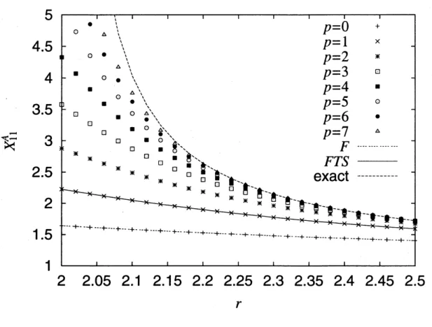
Figure 1: The scalar function $X_{11}^{A}(r)$ of the two-body resistance problem for various case. $‘ F$’ and $‘ FTS$’

show the corresponding values obtained by the analytical expressions and ‘exact’ shows the results by Jeffrey&Onishi (1984). The results by the present formulation

2.5

Higher

version

for

rigid

particles

For the check of the formulation and the implementation,

we

calculate the two-body

re-sistance matrix for $p=0,1,$$\cdots,$$7$ and compare them to the exact solution by [11]. In

addition, we

can

compare the results with the analytical forms of the scalar functions.

Figure 1 shows

one

of the scalar functions in the resistance matrix$X_{11}^{A}(r)$ for various

cases.

The analytical expression of$X_{11}^{A}(r)$ for $F$ version is given by

$X_{11}^{A}(r)= \frac{4r^{6}}{4r^{6}-(3r-22)2}$, (32)

and for $FTS$ version is given by

$X_{11}^{A}(r)= \frac{20r^{6}}{D}(-2880+2208r^{2}-260r^{4}-75r6+20r^{10})$_{, (33)}

where

$D$ $=$ $2304-21120_{r}2+55600r^{4}-90600r6+45945r^{8}$

$-8\mathrm{o}\mathrm{o}_{r^{1}-}01800_{r}12-900_{r}14+400_{r^{16}}$. (34)

This shows that the results of$p=0$ and $p=1$ are completely identical to the analytical results and converge to the exact solution

as

$parrow\infty$.

3

Fast scheme

The bottleneck in the Stokesian Dynamics method is in the inversion of the mobility matrix. Therefore we need to improve the calculation of the linear set of equations faster than

$O(N^{3})$. As suggested by [10], the application of conjugate-gradient type iterative methods

is the first step for the improvement. The iterative method for the Stokesian Dynamics method gives an $O(N^{2})$ scheme at best, consisting only of the calculation of the

dot-product between the mobility matrix and the force moment, which would be the next

bottleneck. The fast multipole method, which is a simple extension of the conventional multipole expansion, is applicable for the calculation and gives

an

$O(N)$ scheme with

a

good convergence.

Before proceedingwe consult the cost of calculation in the six-stepprocedureto seewhere

the next bottleneck is. The steps except for (ii) are the calculation for each particles, and therefore the cost is $O(N)$. On the other hand, the calculation of_{the step (ii) contains the}

FMM is originally developed by [8] for Laplace problem in two- and three-dimensions with non-adaptive tree-structure, and is extendedshortly to adaptive

one

by [3]. The application to the $1\mathrm{o}\mathrm{W}^{-}\mathrm{R}\mathrm{e}\mathrm{y}\mathrm{n}\mathrm{o}\mathrm{l}\mathrm{d}\mathrm{S}$-number flows is shown by [19]. The aim of our formulation of FMM

is to make the scheme for free boundary condition with

a

simple formulation, while $[19]’ \mathrm{s}$

formulation is for periodic boundary condition and is so complicated. We only consider

the non-adaptive scheme in this work.

3.1.1 Outline of FMM

Our aim is now to calculate $\mathcal{V}’(\alpha)$ defined by (25) efficiently. The point of FMM is that

we

treat particles

as a

group not only for $\beta’ \mathrm{s}$ in the force moments $\mathcal{F}(\beta)$ but also for $\alpha’ \mathrm{s}$

in the velocity derivatives $\mathcal{V}’(\alpha)$ in (25). In other words,

we

expand not only $y$ but also $x$

on the integral equation (1).

To make an efficient procedure to calculate the velocity derivatives, we introduce hierar-chical cell-structure and formulate the calculations between the levels of the cell-structure. First we define the primary cell at level $0$ which contains all particles. At the next level 1,

we divide the primary cell into $2^{3}$ cells called ‘children.’ This division is repeated up to the

level $l_{m}$, where the cells are called ‘leaves’. All cells except for leaves have 8 children and

all cells except for the primary cell have their ‘_{parent’ cell.}

Firstwe are going to formulate the basic formulae to shift the origin of the force moments and that of the velocity derivatives, and then, to discuss the concrete implementation of FMM.

3.1.

$\cdot$

2.

$\mathrm{S}\mathrm{h}\mathrm{i}\mathrm{f}\mathrm{t}’$

. -operation of force moments

We describe the transformations of the origin ofmoments here. We would like torepresent the moments with the origin $x_{2}$ by $F(x_{1})$. From the definition, the moments with $x_{2}$ is

given by

$F_{i,k}^{(m)} \ldots(_{X_{2}})=\int dS(y)(y-x_{2})km\ldots fi(y)$

.

(35)

Here $(y-X_{2})^{m}$ could be written by the linear combination of $(y-X1)^{i}$ and $(x_{1}-X_{2})^{j}$

where

$i+j=m$

. By the ‘binomial theorem for 3-dimensional vectors’, we

are

able to

transform $F(x_{1})$ to $F(x_{2})$ uniquely. The point of the binomial theorem for vectors is the

non-commutable property;

$aibj\neq b_{i}a_{j}$. (36)

The expansion ofpower of the

sum

of two vectors $a$ and $b$ is, though, straightforward. We

just write down explicitly for lower powers;

$F_{i,j}^{(1)}(x2)$ _$=$ $r_{j}\mathcal{F}_{i}^{(}(0)x_{1})+F_{i.j}^{(1)}(X1)$

$\mathcal{F}_{i,jk}^{(2)}(x2)$ _$=$ $r_{jk}^{2()}\mathcal{F}_{i}0(x_{\iota}\mathrm{I}+r_{j}F_{i,k}^{(1)}(x_{1})+r_{k}\tau_{i,j(x)}^{(}1)1+\mathcal{F}_{i,jk}^{(2)}(x_{1})$,

(38) (39) where $r=x_{1}-x_{2}$. If the order of$F(x_{1})$ and $\mathcal{F}(x_{2})$ is the same, they

are

equivalent; that

is, $\mathcal{F}(x_{2})$ calculated by.the definition and by the transformation above

are

identical. We

denote this transformation by matrix $S_{F}$

as

$F(x_{2})=S_{F}(x_{2,1}X)\cdot \mathcal{F}(x_{1})$. (40)

3.1.3 shift-operation of velocity derivatives Here we describe the $\mathrm{t}\mathrm{r}\mathrm{a}\mathrm{n}\sim$

.sformation of the origin of velocity derivatives. By the definition

$\mathcal{V}_{i,k}^{(m}..().)X_{1}=\frac{1}{m!}[\nabla^{m}k\cdots v_{i}](X1)$, (41)

the velocity disturbance at $x$ around $x_{1}$ is given by

$v_{i}(x)= \sum_{m=0}\mathcal{V}^{()}i,k\cdot(m..x_{1})(x-X_{1})^{m}k\cdots$. (42)

From the above equation, we get the transformation among the velocity derivatives

as

$\mathcal{V}_{i,l}^{(n.)}..(x_{2})=\sum m=n{}_{m}C_{n}\mathcal{V}_{i}^{(m)},k\cdots l\cdots(x_{1})(x_{2}-x_{1})^{m}k\cdots-n$, (43)

or introducing the operator $S_{V}$ as

$\mathcal{V}(x_{2})=SV(_{X}2, X1)\cdot v(_{X_{1})}.$ (44)

3.1.4 Procedure of FMM

In the calculation of FMM, there are mainly two stages: upward-pass where the force moments of the cells are calculated, and downward-pass where the velocity derivatives of the cells are calculated.

In the upward-pass, we calculate the force moments from particles in the cell $C$

$F(C)= \sum_{\beta\in C}SF(x_{C}, x_{\beta})\cdot F(\beta)$, (45)

for all cells in all levels. This is achieved efficiently

as

follows. First,

we

calculate the force

moment for leaves $L$ directly by the definition (45)

as

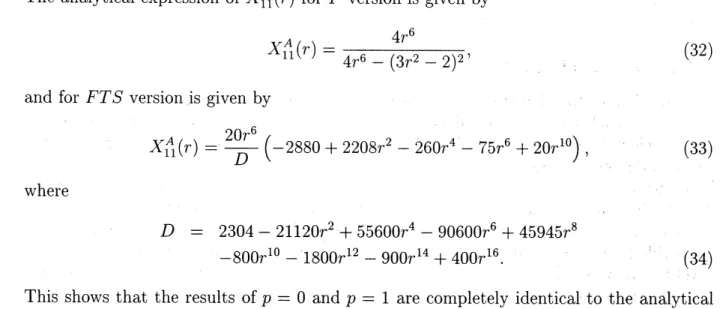
Figure 2: Cell structure in $2\mathrm{D}$. Well-separated cells of cell $C$ is denoted as $W$ and near

cells of cell $C$ including itself is denoted as $N$. Well-separated cells of$C’ \mathrm{s}$ parent cell $P$ is

denoted

as

$W^{P}$ whose children

are

not $W’ \mathrm{s}$.

where $F(\beta)$ is known variable for all particles $\beta$. The force moment of cell $P$ at the level $l$

is calculated by its children $C$ at the level $l-1$ by the shift operator $S_{F}$ as

$F(P)= \sum_{C\mathrm{o}\mathrm{f}P}^{8}S_{F}(XP, Xc)\cdot \mathcal{F}(c)$. (47)

By this recurrent relation, we

can

calculate all force moments at the levels from $l=l_{m}-1$

to 2. It should be noted that the calculated values in the upward-pass is exactly the

same

with that by the definition (4) for the cells in principle, because the transformation of the origin of the moments (40) is exact. This gives a good check for the program.

The errors in this scheme appear at the truncation of the expansion and we have to keep

a

certain condition to get good estimations. For this purpose we introduce the near cells for a cell $C$ denoted by $N^{C}$ which does not satisfy the

$\mathrm{c}\mathrm{o}\mathrm{n}\mathrm{d}\mathrm{i}\mathrm{t}\mathrm{i}_{0}\mathrm{n}..\cdot$ By the near cell

$N^{C}$, we

define well-separated cells $W^{C}$

as

follows;

$\bullet$ $W^{C}$ is at the

same

level of$C$. $\bullet$ $W^{C}’ \mathrm{s}$parent is $N^{P}$.

$\bullet$ $W^{C}$ is not $N^{C}$.

By the definitions, the most important property that the well-separated cells of$C$, those of

$C’ \mathrm{s}$ ancestors, and the

near

cell of _$C$ cover all region of the primary cell without overlap is

satisfied. The typical definition of $N^{C}$ is the nearest-neighbor cells including cell $C$ itself,

so

that there are $3^{3}$ cells at most. We denote this

as

$n_{s}=1$ where $n_{s}$ is the number

of spacing cells to the nearest well-separated cell. Figure 2 shows that the situation in two-dimensional

case

for simplicity. We note that this is not the only choice but we

can

choose $N^{C}$, for example,

as

the cells inside the square centred by $C$ with 5 times size of $C$

$(n_{S}=2)$, where $5^{3}$ cells would be $N^{C}$ and the result would be more accurate.

In the downward-pass, we calculate the velocity derivatives in an efficient way. For this purpose, we introduce the velocity derivatives of the contributions from the $\mathrm{W}\mathrm{e}\mathrm{l}1_{- \mathrm{s}\mathrm{e}_{\mathrm{P}}\mathrm{a}}..\mathrm{r}$ated

cells of $C$ and $C’ \mathrm{s}$ ancestors defined by

$\mathcal{W}(C)=\sum_{\beta\not\in N^{c}}\mathcal{K}(c, \beta)\cdot \mathcal{F}(\beta)$. (48)

First we set

zero

for $\mathcal{W}’ \mathrm{s}$ at level 1 (at least), because the cells at the level has no

well-separated cell. By the transformation (44), we can calculate $\mathcal{W}(C)$ in terms of the parent’s

$\mathcal{W}(P)$ as

$\mathcal{W}(C)=S_{V}(xc, x^{P})\cdot \mathcal{W}(P)+\sum \mathcal{K}(C, W)\cdot F(W^{c}W)$, (49)

where the second term in the $\mathrm{r}\mathrm{i}\mathrm{g}\mathrm{h}\mathrm{t}-\mathrm{h}\mathrm{a}\mathrm{n}\mathrm{d}_{-}\mathrm{s}\mathrm{i}\mathrm{d}\mathrm{e}$is the contribution not included in $\mathcal{W}(P)$.

By this relation, we can calculate $\mathcal{W}$ for all cells at the levels from $l=2$ to $l_{m}$. Finally,

adding the contribution from the particles in the near cells, we get the velocity derivatives for the particle $\alpha$ by

$\mathcal{V}’(\alpha)=S_{V}(x, x\alpha L)\cdot \mathcal{W}(L)+\sum_{N^{L}\beta\in,\beta\neq\alpha}\mathcal{K}(\alpha, \beta)\cdot \mathcal{F}(\beta)$. (50)

3.1.5 Truncation

Generally errorson the multipole expansion is characterized by the order of truncation and the ratio $r/R$ where $r$ is the distance between the

source

and the expansion-point and $R$

is that between the observation-point and the expansion-point. In the FMM procedure,

the ration $r/R$ is completely controlled by the number of spacing cell $n_{s}$ in the hierarchical

cell-structure as

$\frac{r}{R}\leq\frac{\sqrt{3}}{2(n_{s}+1)}$. (51)

If

we

truncate the force moments at the order $q$ in the calculation of (48),

$\mathcal{K}^{(n,m)}$

for

up to $\mathcal{K}^{()}p+2,p+2$_. This is because the resultant mobility problem (23) must bewell-defined.

Ifwe take larger $q$, we get more accurate

$\mathcal{V}’$. However we should note that (25) with the

truncation $p$ is

an

approximation itself. The

error

introduced in (25) is not clear. This is

because we truncate at the same order for interactions among all particles. The truncation

error

would be change due to the configuration; dilute systems

are

moreaccuratethandense

systems with the same truncation. The largest error in (25) would occurred on the nearest pair because $r$ is equal to $a$ and $R$ is minimized there. With $q=2(p+2)$, the standard

choice $n_{s}=1$ on FMM is equivalent to the existence of pair with $R=4/\sqrt{3}\approx 2.31$ which

would be appropriate for dense systems.

3.1.6 Cost-estimation

Now

we

roughly estimate the calculation-cost

on

the above non-adaptive FMM scheme.

Givingforce moments for all particles as a trial values in the iteration, we can calculate by

the following steps:

$\mathrm{i}$. Assign the force moments for leaves _$L$ by (46) with the cost

of $O(N)$.

$\mathrm{i}\mathrm{i}$. Calculate the force moments for cells above by (47) with the cost of

roughly $O(8n_{c})$

where $n_{C}$ is the number of cells in the hierarchy.

$\mathrm{i}\mathrm{i}\mathrm{i}$. Clear $\mathcal{W}$ at level 1 with the cost of$O(1)$

$\mathrm{i}\mathrm{v}$. Calculate $\mathcal{W}$ at the levels from $l=2$ to $l_{m}$ by (49) with the cost of $O(n_{C}(1+n_{W}))$

where $n_{W}$ is the number of well-separated cells for a cell.

$\mathrm{v}$. Calculate the velocity derivatives of particles by (50) with the cost of $O(N(1+n_{L}))$

where $n_{L}$ is the number of particles in a leaf cell.

The cost ofsteps (ii) and (iii) are negligible for large N. $n_{W}$ is constant with N. $n_{C}$ and

$n_{L}$

are

glven

as

$n_{c=} \sum^{l_{m}}8\iota=0\iota_{=}\frac{8^{\iota_{m}+}1-1}{7}$, (52)

$n_{L} \approx\frac{N}{8^{l_{m}}}$, (53)

where we expect that the configuration is homogeneous in the primary cell. If we choose

$l_{m}\approx\log N$, it is expected that $n_{C}$ is $O(N)$ and $n_{L}$ is $O(1)$. Therefore we could calculate $\mathcal{V}’$ for all particles with the cost of $O(N)$.

After the above calculation with five steps, we return to the step (iii) on the six-step

procedure in \S 2.4, and then we get the irreducible velocity moments $\hat{\mathcal{U}}$

corresponding to the trial force moments for the iteration method totally with the cost of $O(N)$.

1

1

1

$\mathrm{O}\mathrm{L}\supset$

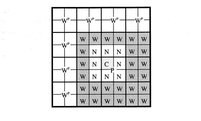
$N$

Figure 3: CPU times with the number of particles $N$. The truncation order in these

calculations is $p=1$ equivalent to $FTS$ version. The truncation order on _{FMM is $q=$}

$2(p+2)$, the number of spacing cell is $n_{s}=1$, and themaximum levels are $l_{m}=2,3,4$ and

5. $‘ FTS$’ _{denotes the conventional Stokedian Dynamics for comparison.}

3.2

Results

Here we utilize the $O(N^{2})$ and the $O(N)$ schemes in practice and check the performance.

The calculations

are

done by personal computer running the FreeBSD operating systemon

dual Pentium III processors of $550\mathrm{M}\mathrm{H}\mathrm{z}$with 1GB memory. The programs are

compi.led

by

the GNU $\mathrm{C}$ compiler optimized for the Pentium processor.

Figure 3 shows the CPU time on the calculation of (23) with the number of particles $N$

for several calculation schemes with $p=1$ which is equivalent to $FTS$ version. The result

denoted by $O(N^{2})$

uses

the six-step procedure in

\S 2.4

and the results denoted by _$O(N)$

use

FMM procedure

on

the step (ii) in the six-step procedure; that is (25). We

see

that the CPU time of $O(N^{2})$ scheme is scaled by $N^{2}$ as expected. For _$O(N)$ scheme with

a

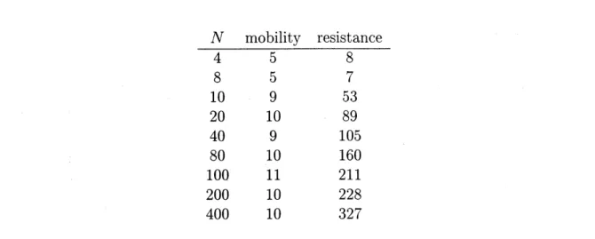
8 57 10 9 53 20 10 89 40 9 105 80 10 160 100 11 211 200 10 228 400 10 327

Table 1: Numbers of iteration for mobility and resistance problems of the simple cubic

configuration in FMM code with $p=1,$ $q=4$, and $l_{m}=2$ by $\mathrm{B}\mathrm{i}\mathrm{C}\mathrm{G}\mathrm{S}\mathrm{T}\mathrm{A}\mathrm{B}2$ method under

the accuracy $10^{-12}$.

fixed$l_{m}$,

we see

two regions where the CPUtime is almost constant with $N$ and where it is

almost scaled by $N^{2}$. The

crossover occurs

where the direct particle-to-particle calculation

for

near

cells with $O(N^{2})$ cost dominates the calculation for cells with $O(N^{0})$ cost for a

fixed $l_{m}$. As suggested in \S 3.1.6, we need to divide the system into finer cells for larger

$N$. In fact larger $l_{m}$ is fast for larger $N$ and the envelope line for $O(N)$ schemes is almost

scaled by $N$. The result denoted by $‘ FTS$’ _{is the calculation with the explicit form} of the

mobilitymatrix shown in [6, Durlofsky et $al.(1987)$]. The generalization for the truncation

$p$ in $O(N^{2})$ scheme makes an extra cost. For higher versions, these behaviours

are

also

observed.

The choice of the schemes is independent from the types of the problem, because all problems-mobility, resistance,and mixed problems-consists of the irreducible generalized mobility equation (23) as the

core.

The total calculating cost depends on the number of iteration. Table 1 shows the number of iteration for mobility and resistance problems in FMM code. This shows that the mobility problem is solved with $O(N)$ cost, but the

resistance problem need more iterations for larger $N$.

4

Conclusions

In this work, wehave shown the formulation of the hydrodynamic interaction among rigid spherical particles in low-Reynolds-number flows with free boundary condition by the mul-tipole expansion in real space and shown the generalized mobility problem which relates

the force moments to the velocity moments. By this formulation,

one

of the difficulties in

truncation beyond $FTS$ version–is overcome. We have also shown the improvement of

the calculating speed which is the other difficulty in the Stokesian Dynamics method. First

we have shown the application of iterative method to solve the linear equations appeared in the highertruncations, and have given the $O(N^{2})$ scheme. Because we calculate not the

velocity moments but the velocity derivatives, the fast multipole method which is a natural extension of the conventional multipole expansioncan be easily applied andwe have shown the non-adaptive versionof the fast multipole method giving the $O(N)$ schemewith agood

convergence.

By thisscheme, the detailed hydrodynamicinteractions for huge conglomerate of particles

in

a

fluid which did not achieved

so

far due to the heavy calculations (for example, the

breakup on falling in [17] and by shear in [12]$)$ are tractable. Not only for this type of

direct application, the formulation would be easily applicable for other problems such as

liquid-liquid systems and for periodic boundary condition, due to the simple formulation.

The adaptive version of the fast multipole method does not discussed in this work, but this would be important for the practical studies, because we usually meet the structures

or the patterns.in the systems and the non-adaptive version hardly handles the situations.

References

[1] BRADY, J. F.

&BOSSIS,

G. 1988 Stokesian dynamics. Annu. Rev. Fluid Mech. 20,

111-157.

[2] BRADY, J. F., PHILLIPS, R. J., LESTER, J. C.

&

BOSSIS, G. 1988 Dynamic simulation of hydrodynamically interacting suspensions. J. Fluid Mech. 195, 257-280.

[3] CARRIER, J., GREENGARD, L.

&

ROKHLIN, V. 1988 A fast

_adapti.ve

multipole

algorithm for particle simulations. J. Comput. Phys. 9, 669-686.

[4] CICHOCKI, B., $\mathrm{E}\mathrm{K}\mathrm{I}\mathrm{E}\mathrm{L}- \mathrm{J}\mathrm{E}\dot{\mathrm{Z}}\mathrm{E}\mathrm{w}\mathrm{s}\mathrm{K}\mathrm{A}$, M. L.,

&WAJNRYB,

E 1999 Lubrication

correc-tions for three-particle contribution to short-time self-diffusion coefficients in colloidal

dispersions. J. Chem. Phys. 111, 3265-3273.

[5] DAMOUR, T.

&IYER,

B. R. 1991 Multipole analysis for electromagnetism and lin-earized gravity with irreducible Cartesian tensors. Phys. Rev. D43, 3259-3272. [6] DURLOFSKY, L., BRADY, J. F.

&BOSSIS,

G. 1987 Dynamic simulation

_,of

hydro-dynamically interacting particles. J. Fluid Mech. 180, 21.

[7] GLUCKMAN, M. J., PFEFFER, R.

&WEINBAUM,

S. 1971 A new technique for

treating multiparticle slow viscous flow: axisymmetric flowpast spheres and spheroids. J. Fluid Mech. 50, 705-740.

Comput. Phys. 73, 325-348.

[9] GUTKNECHT, M. H. 1993 Variants ofBiCGStabfor matrices with complex spectrum.

SIAM J. Sci. Stat. Comp. 14, 1020-1033.

[10] ICHIKI, K.

&BRADY,

J. F. 2000 Many-body effects of matrix-inversion in

low-Reynolds-number hydrodynamics. Phys. Fluids.

[11] JEFFREY, D. J.

&ONISHI,

Y. 1984 Calculation of the resistance and mobility $\mathrm{f}\mathrm{u}\mathrm{n}\mathrm{c}_{-}$

tions for two unequal spheres in $1\mathrm{o}\mathrm{W}^{-}\mathrm{R}\mathrm{e}\mathrm{y}\mathrm{n}\mathrm{o}\mathrm{l}\mathrm{d}\mathrm{s}$-number flow. J. Fluid Mech. 139,

261-290.

[12] KAO, S.

&MASON,

S. G. 1975 Dispersion of particles by shear. Nature 253, 619-621. [13] LADD, A. J. C. 1988 Hydrodynamic interactions inasuspensionofspherical particles.

J. Chem. Phys. 88, 5051-5063.

[14] LADYZHENSKAYA, O. A. 1969 The mathematical theory

_of

viscous incompressible

flow, 2nd edn. Goldon&Breach.

[15] MAZUR, P.

&VAN

SAARLOOS, W. 1982 Many-sphere hydrodynamic interactions and mobilities in a suspension. Physica A 115, 21-57.

[16] Mo, G.

&SANGANI,

A. S. 1994 A method for computing Stokes flow interactions

among spherical objects and its application to suspensions of drops and porous

parti-cles. Phys. Fluids 6, 1637-1652.

[17] NITSCHE, J. M.

&BATCHELOR,

G. K. 1997 Break-up of a falling drop containing

dispersed particles. J. Fluid Mech. 340, 161-175.

[18] SAAD, Y.

&SHULTZ,

M. H. 1986 GMRES-ageneralized minimal residual algorithm

for solving nonsymmetric linear-systems. SIAM J. Sci. Stat. Comput. 7, 856-869.

[19] SANGANI, A. S.

&Mo,

G. 1996 An $O(N)$ algorithm for Stokes and Laplace

inter-$\dot{\mathrm{a}}$

ctions of particles. Phys. Fluids 8, 1990-2010.

[20] VAN DER VORST, H. A. 1992 BI-CGSTAB: A fast and smoothly converging variant

of BI-CG for the solution of nonsymmetric linear systems. SIAM J. Sci. Stat. Comp.

13, 631-644.