Dynamics of Vortical Structure in a Homogeneous Shear Flow(Mathematical Fluid Mechanics and Modeling)

Dynamics

of

Vortical

Structure

in

a Homogeneous

Shear Flow

Shigeo Kida

_TH

$\ovalbox{\tt\small REJECT}$

R

RIMS, Kyoto University

Mitsuru Tanaka

ffl

$\mathbb{E}$

P

$|$

E

Faculty of Science, Kyoto University

1.

Introduction

The coherent structures, suchastubesand layers of concentratedvorticity,observed

in fully developed turbulence have relativelylong lifetimes. They are considered to play

an essential role in turbulence dynamics. For example, the longitudinal vortex tubes

oriented nearly along the mean flow direction play an important role in the production

ofturbulenceenergy in wall turbulence. Regeneration mechanism of longitudinal vortex

tubes have been extensively investigated for this reason.(1-4) _{But their dynamics is not}

wellunderstood yet and should be explored furthermore.

Here weconsider a homogeneous shear flow, which is one of the simplest flows with

non-zero mean flow profile. This would enable us to investigate vortical structures in

detail. Several direct numerical simulations(5-9) _{revealed that vortical structures that}

are quite similar to those observed in a wall turbulence prevail also in homogeneous

shear turbulence. Rogers and Moin(6) _{observed a hairpin-shaped vortical structure in}

a homogeneous shear flow with relatively weak strain. Lee et $al^{(7)}$ made comparisons

with the turbulent channel flows and found that if the mean shear rate is as strong as

that in the buffer layer of a wall turbulence, the streak structures can appear even in the

absence of a solid wall. There also exist longitudinal vortex tubes and vortexlayers(8,9)

which are observed in the wide rangeofshear strength and Reynolds number. Roughly

speaking, there are two types ofregeneration mechanisms of longitudinal vortex tubes

in wall turbulence. One is phenomena which take place at a wall. The other is the

inviscid one which may be attributed to the existence of a shear. In the research of

homogeneous shear flows we can investigate the effects of shear on the generation of

longitudinal vortex tubes separatelyfrom those of a wall.

In the present report we focus an attention to the vortical structures in a

them. In

\S 2

we briefly describe our numerical simulations.$\cdot$

We examine the statistical

properties of vorticity vectors in

\S 3

and interactions betweenlongitudinal vortex tubes

and vortex layers in

\S 4.

2. Numerical

Simulation

2.1 Basic Equation

We consider the motion of an incompressible viscous fluid in a linear mean shear

$U=(Sx_{2},0,0)$, (1)

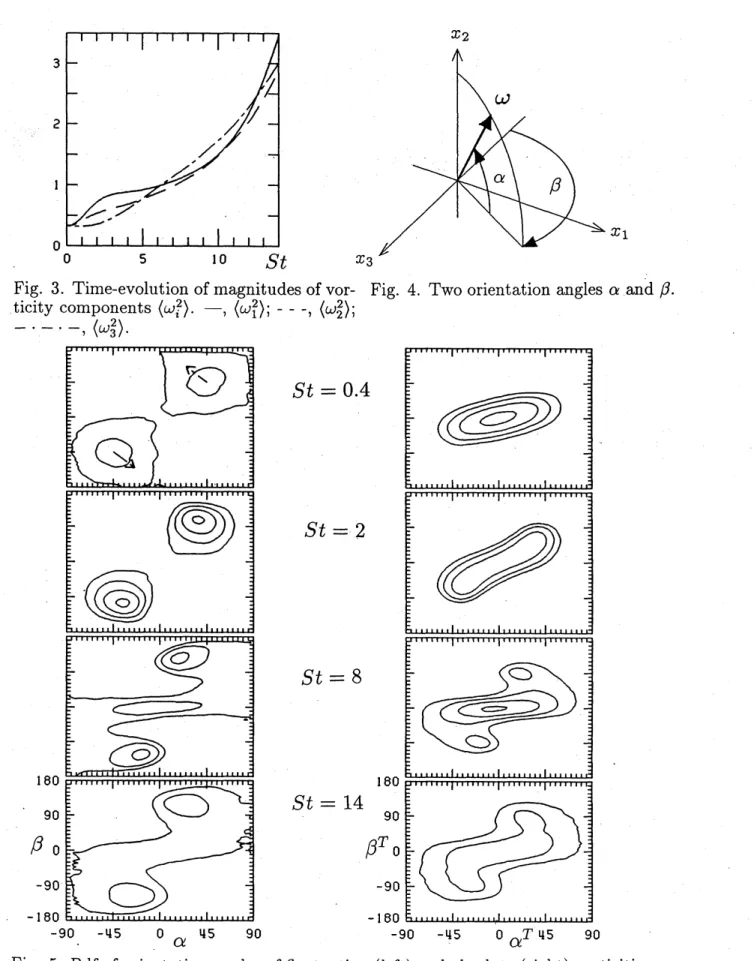
which is along the $x_{1}$-direction andvaries linearly with $x_{2}$ (Fig. 1). The mean vorticity

$\Omega$ is therefore uniform in space and is directed toward the negative

$x_{3}$-axis, that is

$\Omega=(0,0, -S)$

.

(2)

Here, we call the $x_{1}-,$ $x_{2}$-and $x_{3}$-axes the streamwise, vertical, and spanwisedirections,

respectively. Time-evolution of the fluctuating velocity $u$ is described by the

Navier-Stokes equation

$\frac{\partial u_{i}}{\partial t}+Sx_{2}\frac{\partial u_{i}}{\partial x_{1}}+Su_{2}\delta_{i1}+uk\frac{\partial u_{i}}{\partial x_{k}}=-\frac{\partial p}{\partial x_{i}}+\nu\nabla^{2}u_{i}$ , $(i=1,2,3)$ (3)

supplemented by the continuity equation $\partial u_{j}/\partial x_{j}=0$, where $p$ is the pressure and $\nu$

is the kinematic viscosity of afluid. Thefluid density is assumed to be uniform and be

unity. A summation is taken over 1–3 for repeated subscripts.

By taking the curl of (3), we obtain the equation for the fluctuating vorticity

$(\omega=\nabla\cross u)$

$\frac{\partial\omega_{i}}{\Re}=-(Sx_{2}\frac{\partial\omega_{i}}{\partial x_{1}}+uk\frac{\partial\omega_{i}}{\partial x_{k}})+(S\omega_{2}\delta_{i1}-S\frac{\partial u_{i}}{\partial x_{3}}+\omega_{k}\frac{\partial u_{i}}{\partial xk})+\nu\nabla^{2}\omega_{i}$. (4)

The first and the second terms in the first brackets on the rhs of (4) represent the

advectionof vorticity bythemean shearandthefluctuatingvelocity, respectively. Three

terms in the second brackets describe a conversion offluctuating vorticity by the mean

shear, a conversion of the mean vorticity by the fluctuating field, and a conversion

of fluctuating vorticity by the fluctuating field, respectively. Finally, the last term

represents viscous diffusion.

Equation (3) is solved numerically in acoordinate systemwhich is advected by the

mean

flow.(5) _{The computation is carried out on 12}$8^{}$ grid points in a rectangular box of

sides $4\pi\cross 2\pi\cross 2\pi$ by using the Fourier spectral_$/Runge$-Kutta-Gill scheme. The initial

velocityfield is givenwith Fourier coefficientswithrandom phase and with a prescribed

energy spectrum of form $E(k)=ck^{4}\exp[-2k^{2}/k_{0}^{2}]$, where $c$ and $k_{0}$ are constants.

There are two non-dimensional parameters that characterize this problem. The

shear rate parameter

$S^{*}= \frac{u^{\prime 2}/\epsilon}{1/S}$

represents the ratio of the time-scale of the nonlinear interaction and that of the mean

shear.(7) _Here, $u’$ is the rms offluctuating velocity and $\epsilon$ is the mean energy dissipation

rate. The Reynolds number

$R_{\lambda}= \frac{u^{\prime 2}/\epsilon}{1/\omega}$

represents the ratio of the time-scaleof the nonlinearinteraction and that of the viscous

effects, where$\omega’$ is the rms of vorticity. We here report the numerical results for

$S^{*}(0)=$

$16$ and $R_{\lambda}(0)=16^{(8,9)}$ The ratio of the rms ofvorticity and the shear rate is 1 at the

initialinstant and therefore the mean strain and the nonlinear self-interaction may play

comparable roles.

3.

Vortical Structures and

Vorticity

Vectors

3.1 Vortical Structures in Homogeneous Shear Turbulence

Many complicated vorticalstructures develop and interact with each other in

homo-geneous shear turbulence. There are three typical vortical stmctures; the longitudinal

vortex tubes nearly along to the streamwise direction, the lateral vortex tubes along

the spanwisedirection, and the vortex layerswith spanwise vorticity. Here, the vortical

structures are regarded as concentrated regions ofvorticity.

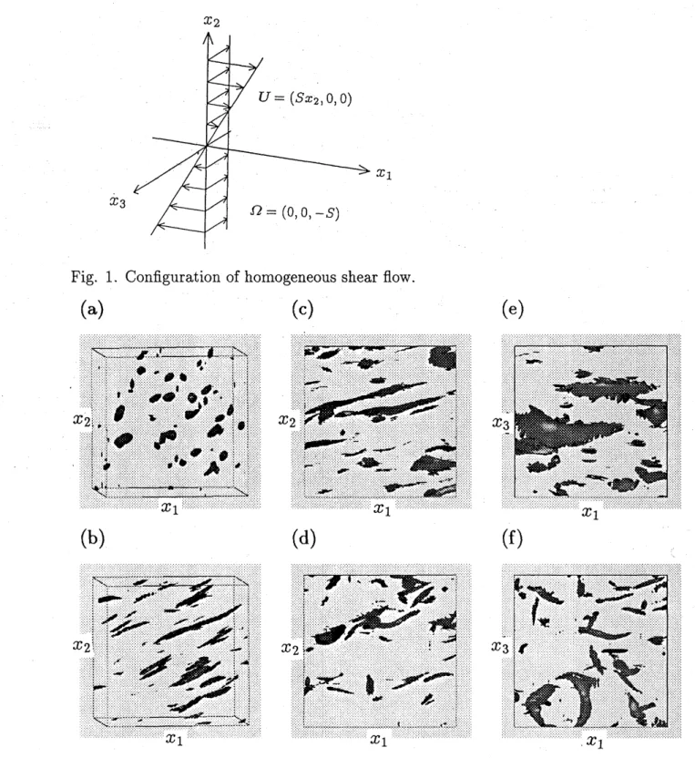
The spatial structure of vorticity field is visualized with the iso-surface ofvorticity

magnitude. In Figs. 2 we plot iso-surfaces at $St=0.4,2,8,14$inacubic domain of sides

$2 \pi\cross\frac{80}{128}$. The iso-surfaces at $St=8$ and $St=14$ are also seen

from.the

$x_{2}$-direction in

Figs.(e) and (f), respectively. The vorticity field is isotropic at the initial instant and

regions of relativelyhigh vorticity are seenas vorticity blobs(figuresomitted). At earlier

times $(St=0.4)$ high-vorticity blobs are being stretchedin the direction inclined at $45^{o}$

to the downstream. Elongated high-vorticity regions are clearly seen at $St=2$

.

These

the longitudinal vortex tubes incline more toward the streamwise direction. As shown

in Figs. 2(c) and 2(e) high-vorticity regions at $St=8$ exhibit layer-like structures.

These vortex layers extend over several ten mesh-sizes in the streamwise direction and

nearly ten mesh-sizes in the spanwise. Vorticity vectors in the layers are directed along

the negative spanwise axis, that is, the direction of the mean vorticity. These vortical

structures break down at further later stages (Fig. $2(e)$). Lateral vortex tubes along

the spanwise direction are also seen in Fig. 2(f).

Figure 3 shows the time-evolution of magnitude of each component of vorticity

$\langle\omega_{i}^{2}\rangle,$$i=(1,2,3)$, where $\{$ $\}$ denotes the spatial average. Enstrophy $\omega^{;2}=\sum\langle\omega_{i}^{2}\rangle$

increases almost exponentially in time, whereas the behavior of each element is quite

complicated. In early stages $(0\leq St\leq 2)$ thestreamwisecomponent$\langle\omega_{1}^{2}\}$ growsrapidly,

which represents the generation and development oflongitudinal vortex tubes. In this

period the spanwise component $\langle\omega_{3}^{2}\rangle$ is almost invariant in time since vorticity lines are

not directly stretched in the spanwise direction by the mean shear. In the subsequent

period$(2\leq St\leq 5)$ the streamwise component increases only slowly in time, suggesting

that the development of longitudinal vortex tubes are balancedagainstviscous diffusion.

The spanwise component, on the other hand, exhibits a rapid growth after $St=2$,

which corresponds to the development of the vortex layers. As will be discussed in

\S 4,

the spanwise component of vorticity is generated from the shear vorticity through

a spanwise vortex stretching and therefore has the same sign as the mean vorticity.

A rapid increase of the spanwise component is followed by a second rapid growth of

the streamwise component. Finally, the streamwise component becomes larger thanthe

spanwise. Longitudinal vortex tubes and vortex layers are observed as dominant vortical

stmctures in the earlier stage $(0\leq St\leq 6)$ and in the middle stage $(6 \leq St\leq 12)$,

respectively, as indicated by the fact that the streamwise and spanwise components are

the largest vorticity in the respective stages. At a further later stagelongitudinal

vortex

tubes constitute the dominant structures again.

Wehave observed the following scenario ofgeneration, development and breakdown

of vortical structures (see ref. (9)).

(i)The linear mean shear flow stretches a randomly distributed initial vorticity field

to generatelongitudinal vortex tubes. Theselongitudinalvortex tubes are subsequently

inclined more and more toward the streamwise direction increasing their strength.

Vor-ticityvectors inside longitudinal vortex tubes are less inclined than the tubes themselves.

which

stretches fluid elements in the spanwise direction most effectively to generate

vortex

layers with spanwise vorticity. Vortex layers are observed to be wrapped into

longitudinal vortex tubes.

(iii) These vortex layers roll up into the lateral vortex tubes through the

Kelvin-Helmholtz

instability. These lateralvortextubes arestretchedanddeformedinto hairpin

vortextubes and longitudinal vortex tubes by themean shear.

(iv) All of these typicalstructures break downinto adisordered weak vorticity field

through some instability mechanisms and complicated mutual-interactions.

Among these four processes, (ii) and (iii) are expected to play important roles in

the formation of vortical structures, that is, longitudinal vortex tubes are intensified

and regenerated by these processes. In the following we pay a special attention to the

process (ii), that includes interactions between longitudinal vortex tubes and vortex

layers.

3.2 Statistical Properties ofVorticity Vectors

In order to examine the distribution of direction of the vorticity vector

quantita-tively we introduce two orientation angles $\alpha$ and $\beta$, which are called the vertical and

horizontal angles, respectively (Fig. 4). We have the following relations,

$\{\begin{array}{l}\omega_{1}=\omega\cos\alpha\sin\beta,\omega_{2}=\omega\sin\alpha,\omega_{3}=-\omega\cos\alpha\cos\beta,\end{array}$ (5)

where $\omega=|\omega|$. Note that the origin $(\alpha, \beta)=(0^{o}, 0^{o})$ corresponds to the negative

$x_{3}$-axis, $i.e$

.

the direction of vorticity of the mean shear.

Suppose that $P(t,\omega)$ is a probability density function (pdf) of vorticity vectors $\omega$

at time$\backslash t$. A pdf of the orientation angles ofvorticity(6) weighted by $\omega^{2}$ is giveby

$f(t, \alpha, \beta)\equiv c\int_{0}^{\infty}\omega^{2}P(t,\omega)\omega^{2}d\omega$, (6)

where $c$ is a normalization factor.

The change in time of vorticity vectors maygivehelpful informationfor

understand-ing of the dynamics of vortical stmctures. The time-evolution of the pdf is described

by

where $D\omega/Dt$ denotes the Lagrangian derivative ofvorticity vectors which is calculated

through the vorticity equation (4). The time-evolution of the pdfoforientation angles

is represented in the spherical coordinate system $(\omega, \alpha, \beta)$ by the equation

$\frac{\partial}{\partial t}f=2g_{\omega}-\frac{1}{\cos\alpha}\{\frac{\partial}{\partial\alpha}(g_{\alpha}\cos\alpha)+\frac{\partial}{\partial\beta}g\beta\}$, (7)

where

$g(t, \alpha,\beta)\equiv c\int_{0}^{\infty}\omega\frac{D\omega}{Dt}P\omega^{2}d\omega$ (8)

expresses the statistical change in time of direction of vorticity vectorspointing to the

direction of$\omega$

.

Notice that 2$g_{\omega}$ represents the change in time ofmagnitude of vorticity

vectors, that is, the production rate of enstrophy.

Inorder to get information about the change in time of direction of vorticity vectors

we take time-derivatives of(5) to obtain the relationship between the time-derivative of

vorticity vectors and orientation angles $(\alpha, \beta)$,

$\frac{D\alpha}{Dt}=\frac{1}{\omega}(-\frac{D\omega_{1}}{Dt}\sin\alpha\sin\beta+\frac{D\omega_{2}}{Dt}\cos\alpha+\frac{D\omega_{3}}{Dt}\sin\alpha\cos\beta)$,

$\frac{D\beta}{Dt}=\frac{1}{\omega\cos\alpha}(\frac{D\omega_{1}}{Dt}\cos\beta+\frac{D\omega_{3}}{Dt}\sin\beta)$ .

The movement ofindividual orientation angles may be expressed by the pdf of $D\alpha/Dt$

and $D\beta/Dt$ weighted by $\omega^{2}$ as

$\frac{d\alpha}{dt}\equiv\int_{0}^{\infty}\omega^{2}\frac{D\alpha}{Dt}\omega^{2}d\omega=n_{\alpha}\cdot g$, $\frac{d\beta}{dt}\equiv\int_{0}^{\infty}\omega^{2}\frac{D\beta}{Dt}\omega^{2}d\omega=n_{\beta}\cdot g$, (9)

where $n_{\alpha}=(-\sin\alpha\sin\beta, \cos\alpha, \sin\alpha\cos\beta)$ and $n_{\beta}=(\cos\beta, 0, \sin\beta)/\cos\alpha$ in the physical

coordinate.

In Fig. 6 we show the weighted pdf of orientation angles of vorticity at $St=$

0.4, 2, 8, 14 (Eq(6)). The pdf’s for the fluctuating and the absolute vorticitiesareplotted

in the left and the right sides, respectively. Here, the absolute vorticity is defined as

$\omega^{T}=\Omega+\omega=(\omega_{1},\omega_{2},\omega_{3}-S)$

.

The distribution is symmetric with respect to the

origin, whichreflects theinvananceof the flowconfiguration by arotation ofangle $180^{o}$

around the $x_{3}$-axis. The pdf is normalized so that the integral over the whole angle

takes unity. Contour levels are 1, 2, 4,$\cdots$

.

First, we discuss the pdf for the fluctuating vorticity. At earlier times $(St=$

maximal

expansion of the mean shear $(Sx_{2},0,0)^{(6)}$ As time goes on, the peaks become sharper, representing longitudinal vortices are being generated. They move toward

$(\alpha, \beta)=(0^{o}, \pm 180^{o})$

.

The decrease of $|\alpha|$ represents that the fluctuating vorticity tends

toincline toward the streamwise direction, while the increase of$|\beta|$ means that they are

turned

to the opposite to the vorticity of the mean shear. A mechanism of the change

in direction of vorticity vector were investigated in ref. (9). The positions of the peaks

eventually stay around $(\alpha_{peak}, \beta_{peak})=\pm(20^{o}, 130^{o})$. These statistically equilibrium

angles should be maintained by some complicated dynamics of vortical

structures.

In a later period there appears two peaks at $(\alpha_{peak}^{T}, \beta_{peak}^{T})=\pm(20^{o}, 90^{o})$in the pdf

for the absolute vorticity, which also corresponds to the longitudinal vortex tubes. It

is interesting that the horizontal peak angle $\beta_{peak}^{T}$ is $\pm 90^{o},$ $i.e$

.

the absolute vorticity

in the longitudinal vortex tubes are aligned perpendicularly to the mean vorticity. No

clear-cut explanation exists, however.

Inthe pdf for fluctuating vorticity there appears another peak around the origin at

$St=8$, which disappears at $St=14$

.

_{This peak corresponds to vortex layers generated}

around this period (see

_{\S 4).}

Vorticity vectors corresponding to this peak are pointed

to the direction of the mean shear vorticity. This peak is thin in horizontal angle $\beta$

and wide in vertical angle $\alpha$, which reflects wavy vortex layers in which the vorticity is

perpendicular to longitudinal vortex tubes.

Next, we examine the change in time of vorticity vectors. We consider the pdf

for absolute vorticity. In Fig. 6(a) we plot the production rate of enstrophy 2$g_{\omega}$ at

$St=8$

.

Positive regions are shaded. The pdf is normalized so that the total volume

takes unity as in the pdf of orientation angles. Note that $D\omega^{2}/Dt>0$ (see Fig. 3).

Contour levels are 1, 2,4, $\cdot\cdot,$$-1,$ $-2,$

$\cdot\cdot$. Vorticity is strengthened in the positive region

around the origin and is weakened in negative regions around the peaks corresponding

to the longitudinal vortex tubes $(\alpha, \beta)=(\pm 20^{o}, \pm 90^{o})$. The pdf takes very large values

at the origin, which means that vorticity vectors oriented in the direction of the mean

vorticity are most effectively stretched. On the other hand, the magnitude of vorticity

vectors in longitudinal vortex tubes tends to decrease in time. In fact, the stretching

termsin the second brackets in the rhs of (4) amplify inaverage all the vorticity vectors.

In thenegative regions, however, the effect of viscosity dominatesthat ofthe stretching.

Now,we consider thechangein timeofdirectionof vorticityvectors. In Fig. 6(b) we

plot the pdfof time-derivative field $(d\alpha/dt, d\beta/dt)$ of the orientation angles at $St=8$.

vectors. Contour lines of the pdf of the orientation angles are shown for reference (see

Fig. 5). The flow in the vectorfield has a peculiar feature. It migrates from the origin

to the right and left along a line $\beta^{T}=0$ up to $|\alpha^{T}|=40^{o}\sim 90^{O}$. Then the flow changes

its direction toward larger $|\beta^{T}|$ until $|\beta^{T}|=90^{o}\sim 120^{o}$

.

Remember that the pdf ofthe

orientation angles has peaks at $(\alpha_{peak}^{T}, \beta_{peak}^{T})=\pm(20^{o}, 90^{o})$ which roughly represents

the mean orientation of longitudinal vortex tubes. The flow tums around these peaks

and approaches $(\alpha_{peak}^{T}, \beta_{peak}^{T})=\pm(0^{o}, 90^{o})$

.

This flow pattem is commonly observed at

other times $(St>2)$

.

Figure 6(c) illustrates the change in time ofvorticity vectors in the physical space.

Here, solid and blank arrows denote the directions of vorticity vectors and their

time-evolution. First, the vorticity vectors oriented to the direction of the mean vorticity

are inclined toward the $x_{2}$-direction. After they are inclined at $40^{o}\sim 90^{o}$ to the

neg-ative spanwise direction, they start turning toward the positive $x_{3}$-direction, $i.e$

.

the

opposite to the mean vorticity. While the spanwise component of absolute vorticity

$\omega_{3}^{T}$ approaches zero, it begins to lean toward the

$x_{1}$-direction. Taking the results in

Figs. 6(a) and 6(b) into account, weunderstand that the vorticity generated around the

direction of the mean vorticity is transferred to the streamwise direction and is

dissi-pated there. Equation (7) gives the change in time of the pdf of the orientation angles.

The first and the second terms in the rhs of (7) represent the contribution from vortex

stretchingand tilting, respectively. Thefirst termdominates the second around the

ori-gin, whereas they are comparable around the peaks corresponding to the longitudinal

vortex tubes.

4.

Interactions

between

Longitudinal

Vortex Tubes and Vortex

Layers

4.1 Development of Vortex Layers due to PairsofLongitudinalVortex Tubes

We consider here a mechanism of generation of vortex layers which are observed

in the iso-vorticity surfaces $($Fig. $2(c,$ $e))$. Figure 7 illustrates a generation mechanism.

Longitudinal vortex tubes induce straining flows perpendicular to themselves. These

straining flows distort the vorticity field in a random way, which in average stretches

fluid elements. The spanwise component of absolute vorticity dominates the other

components, since the mean vorticity is along the negative spanwise axis. Therefore, the

stretchingin the spanwise direction maymost effectively contribute to magnify vorticity

an extremely strong spanwise expansion can be generated by combined effects of two

pairs of vortex tubes arranged as shown schematically in Fig. 7. If they happen to

be arranged in this way, a strong vortex layer with spanwise component of vorticity is

generated

between them. In Figs. 8 we plot the streamwise vorticity $\omega_{1}$ on the $(x_{3}, x_{2})$

plane. It is positive (in clockwise rotation) in white regions, while it is negative (in

counterclockwise rotation) in dark regions. The vorticity and velocity perpendicular to

the plane are represented bylines in Figs. 8(a) and 8(b), respectively. A thin horizontal

region of concentrated vorticityin the center of Fig. 8(a) represents the cross-section of

a large vortex layer seen in Fig. 2(e). It is clearly seen that the vortex layer is being

intensified due tothe strainingflows (spanwise expansion) induced byfour(twonegative

and two positive) longitudinal vortex tubes.

4.2 Wrapping of Vortex Layer into Longitudinal Vortex Tube

Themovement of vorticity vector as shown in Fig. 6(c) may represents awrapping

process of vortex layers intolongitudinalvortex tubes. In Figs. 9 we sketch a longitudinal

vortex tube and a vortex layer. Figure 9(b) represents a cross-section of the structure.

The longitudinal tube and the layer are oriented nearly to the streamwise direction

(see Figs. 2). The mean flow comes out of the page and the mean vorticity points to

the right. As shown in Fig. 5 the absolute vorticity vectors point to the direction of

the mean vorticity in the vortex layer and are nearly aligned with the structure in the

longitudinal vortextube. The layeris deformed by the flow induced by the longitudinal

vortex tube as shown in Fig. 9(b). At the same time vorticity vectors in the layer are

turned toward the $x_{2}$-direction and then to the positive $x_{3}$-direction. The mean flow

increases vertically, which inclines the vorticity vectors toward the $x_{1}$-direction (see also

a discussion in

\S 5).

This is typically an inviscid phenomenon (remember that vorticity

lines are material in an inviscid fluid). Such behavior of vorticity vectors is consistent

with the change illustrated in Fig. 6(c). In short, vorticity vectors are tilted toward the

streamwise direction rotating around the longitudinalvortex tubes.

It is seen in Figs. 8 that a vortex layer in the center is being wrapped into a

longitudinalvortex tube, one of the fourvortextubes that contribute to the development

of the vortex layer. A three dimensional view of Figs. 8 is drawn in Fig. 10. Grey

regions $(\omega_{3}^{T}\leq-5S)$ and black regions $(\omega_{1}\leq-3.2S)$ correspond to the vortex layer

and the strongest longitudinal vortex tube in Fig. 8, respectively. Black lines represent

the absolute vorticity lines starting at points in the vortex layer which are denoted by

that the flow configuration is invariant under a $180^{o}$-rotation around $x_{3}$-axis. It is

clearly seen that inside the vortex layer vorticity lines are tilted toward the $-x_{2^{-}},$ $x_{3^{-}}$,

and then to the $-x_{1}$-directions. A similar behavior of vorticity lines is observed in a

turbulent boundary

layer.(1)

5. Summary and

Discussions

We have examined interactions between longitudinal vortex tubes and vortex

lay-ers. Longitudinal vortex tubes induce straining flows around them, which stretches

fluid elements in the spanwise direction most effectively to generate vortex layers with

spanwise vorticity. An extremely strong spanwise expansion of fluid elements can be

induced effectively by combined effects of two pairs of vortex tubes arranged as shown

schematically in Fig. 7. Most ofspanwise vorticilyis created by this process. Since

lon-gitudinal vortex tubes induce swirling motions perpendicular to themselves, vorticity

lines thus stretched are tilted toward the $x_{2}$-direction. Generation of vertical vorticity

$\omega_{2}$ is mainly due to the rotation of vorticity lines (in vortexlayers) around longitudinal

vortex tubes. Since the mean shear converts vorticity from the vertical to the

stream-wise components (see thefirst term in the second brackets in the rhs of(4)), the vertical

vorticity may be regarded as a source of the streamwise vorticity.

The generation mechanism of the streamwisevorticity, however, seems to be quite

complicated. Suppose that longitudinal vortex tubes are aligned along the direction

inclined at $\alpha\approx 20^{o}$ to the streamwise axis. We introduce a new coordinate system

$(x_{s}, x_{n}, x_{3})$ along the structure. The time-evolution of the structural component of

vorticity$\omega_{\theta}$ is governed by

$\frac{D\omega_{s}}{Dt}=S(\omega_{s}\sin\alpha\cos\alpha-\omega_{n}\sin^{2}\alpha-\frac{\partial u_{3}}{\partial x_{s}}\cos^{2}\alpha)+\omega_{s}\frac{\partial u_{s}}{\partial x_{s}}-\frac{\partial u_{s}}{\partial x_{n}}\frac{\partial u_{3}}{\partial x_{s}}+\frac{\partial u_{s}}{\partial x_{3}}\frac{\partial u_{n}}{\partial x_{s}}+\nu\nabla^{2}\omega_{s}$

.

(10)

If the fluctuating field is uiiiform in the structural direction, eq.(10) is reduced to

(ne-glecting the viscous term)

$\frac{D\omega_{s}}{Dt}=S\omega_{1}\sin\alpha$. (11)

This tells us that the structural component ofvorticity can be created only if vortical

stmctures (vortex layers) contain the streamwise component of vorticity. Therefore,

a conversion of vorticity from vertical to streamwise components should be caused by

non-uniformityinthe $x_{s}$-directionratherthanthe vertical inclination of thestructureto

role, especially in the regions oflarge$\omega_{2}$ which corresponds wavy vortex layers. Vortex

layers deformed as shown in Fig. 9(b) may be stretched in the streamwise direction by

this term, when they are modulated in the streamwise ($\approx$ structural) direction or are

kinked in the spanwise direction.

It is desirable to examine how the growth of $\omega_{1}$ leads to the generation of

lon-gitudinal vortex tubes. There are several regeneration processes of longitudinal tubes

observed so far: awrapping of vortex layers into longitudinal vortextubes,(1) a roll-up

of vortex layers into lateral vortex tubes and their subsequent deformation to hairpin

vortices,(4,9) a roll-up of vortex layers in which streamwise component of vorticity is

magnified while they are inclined toward streamwise direction.(10) _{It may be of primary}

importance to verify which one is dominant.

References

(1) _{J. Jim\’enez and P. Moin, “The minimal flow unit in near-wall turbulence,” J. Fluid}

Mech. 225 (1991) 213.

(2) _{J.W. Brooke and T.J. Hanratty, “Origin of turbulent-producing eddies in a channel}

flow,” Phys. Fluids A 5 (1993) 1011.

(3) _{P.S. Bernard, J.M. Thomas and R.A. Handler, “Vortex dynamics and the production}

of Reynolds stress,” J. Fluid Mech. 253 (1993) 385.

(4) _{N.D. Sandham and L. Kleiser, “The late stages of transition to turbulence in channel}

flow,” J. Fluid Mech. 245 (1992) 319.

(5) _{R.S. Rogallo, “Numerical experiments in homogeneous turbulence”, NASA Tech.}

Memo. 81315 (1981).

(6) _{M.M. Rogers and P. Moin, “The stmcture of the vorticity field in homogeneous}

turbulence flows”, J. Fluid Mech. 176 (1987) 33.

(7) _{M.J. Lee, J. Kim, and P. Moin, “Structure of turbulence at high shear rate”, J. Fluid}

Mech. 216 (1990) 561.

(8) _{S. Kida and M. Tanaka, “Reynolds stress and vortical structure in a uniformly}

sheared turbulence”, J. Phys. Soc. Jpn. 61 (1992) 4400.

(9) _{S. Kida and M. Tanaka, “Dynamics of vortical structures in a homogeneous shear}

flow”, J. Fluid Mech. (1994) (in print).

(10) _{J. Jim\’enez and P. Orlandi, “The rollup of a vortex layer near a wall”, J. FluidMech.}

Fig. 1. Configuration of homogeneous shear flow.

$($

a

$)$ $($

c

$)$ $($

e

$)$

(b)

(d)

(f)

Fig. 2. Iso-surfaces of vorticity magnitude. (a) $St=0.4,0\leq x_{1}/\triangle x_{1}\leq 40,0\leq x_{2}/\triangle x_{2}\leq$

$80_{0\leq x_{3}/\triangle x_{3}\leq 80}80^{0\leq x_{3}/\triangle x_{3}\leq 80,|\omega}|_{\omega|=32S=2.5\omega,(c)St=8,65\leq x_{1}/\triangle x_{1}\leq 105_{7}40\leq}^{=2.2S.=2.2\omega’,(b)St=2,20\leq x_{1}/\triangle x_{1}\leq 60,0\leq x_{2}/\triangle x_{2}\leq}$

$x_{2}/\triangle x_{2}\leq 120,30\leq x_{3}/\triangle x_{3}\leq 110,$ _{$|\omega|=4.5S=2.4\omega’,$ $(d)St=14,45\leq x_{1}/\triangle x_{1}\leq$}

$85,47\leq x_{2}/\triangle x_{2}\leq 127,47\leq x_{3}/\triangle x_{3}\leq 127,$ $|\omega|=8.9S=3.0’\omega$‘. Iso-surfaces at (e)

$x_{2}$

Fig. 3. Time-evolution of magnitudes ofvor- Fig. 4. Two orientation angles $\alpha$ and $\beta$

.

ticity components $\langle\omega_{i}^{2}\rangle$. –, $\langle\omega_{1}^{2}\rangle;---,$ $\langle\omega_{2}^{2}\rangle$;

-. _$–$

.

$-,$ $\langle\omega_{3}^{2}\rangle$.

Fig. 8. Distribution of$\omega_{1}$ in the $(x_{3}, x_{2})$ plane with (a) the vorticity and (b) the velocity

(b)

Fig. 9. Sketch of wrapping ofa vortex layer into a longitudinal vortex tube.

Fig. 10. Three dimensional view of wrapping of vortex lines. $St=8$. Black and

grey

represent regions $\omega_{1}\leq-3.2S$ and $\omega_{3}^{T}\leq-5S$, respectively. $8\leq x_{1}/\triangle x_{1}\leq 25,0\leq$