JAIST Repository: Auditory-Inspired End-to-End Speech Emotion Recognition Using 3D Convolutional Recurrent Neural Networks Based on Spectral-Temporal Representation

Japan Advanced Institute of Science and Technology

JAIST Repository

https://dspace.jaist.ac.jp/

Title

Auditory-Inspired End-to-End Speech Emotion

Recognition Using 3D Convolutional Recurrent

Neural Networks Based on Spectral-Temporal

Representation

Author(s)

Peng, Zhichao; Zhu, Zhi; Unoki, Masashi; Dang,

Jianwu; Akagi, Masato

Citation

2018 IEEE International Conference on Multimedia

and Expo (ICME): 1-6

Issue Date

2018-07-26

Type

Conference Paper

Text version

author

URL

http://hdl.handle.net/10119/15481

Rights

This is the author's version of the work.

Copyright (C) 2018 IEEE. 2018 IEEE International

Conference on Multimedia and Expo (ICME), 2018,

DOI:10.1109/ICME.2018.8486564. Personal use of

this material is permitted. Permission from IEEE

must be obtained for all other uses, in any

current or future media, including

reprinting/republishing this material for

advertising or promotional purposes, creating new

collective works, for resale or redistribution to

servers or lists, or reuse of any copyrighted

component of this work in other works.

AUDITORY-INSPIRED END-TO-END SPEECH EMOTION RECOGNITION USING 3D

CONVOLUTIONAL RECURRENT NEURAL NETWORKS BASED ON

SPECTRAL-TEMPORAL REPRESENTATION

Zhichao Peng

, Zhi Zhu

, Masashi Unoki

, Jianwu Dang

, Masato Akagi

1

_{Graduate School of Advanced Science and Technology, Japan Advanced Institute of Science and}

Technology, Ishikawa, Japan

2

_{School of Computer Science and Technology, Tianjin University, Tianjin, China}

{zcpeng, zhuzhi, unoki, jdang, akagi }@jaist.ac.jp

ABSTRACT

The human auditory system has far superior emotion recognition abilities compared with recent speech emotion recognition systems, so research has focused on designing emotion recognition systems by mimicking the human auditory system. Psychoacoustic and physiological studies indicate that the human auditory system decomposes speech signals into acoustic and modulation frequency components, and further extracts temporal modulation cues. Speech emotional states are perceived from temporal modulation cues using the spectral and temporal receptive field of the neuron. This paper proposes an emotion recognition system

in an end-to-end manner using three-dimensional

convolutional recurrent neural networks (3D-CRNNs) based on temporal modulation cues. Temporal modulation cues contain four-dimensional spectral-temporal (ST) integration representations directly as the input of 3D-CRNNs. The convolutional layer is used to extract high-level multiscale ST representations, and the recurrent layer is used to extract long-term dependency for emotion recognition. The proposed method was verified on the IEMOCAP database. The results show that our proposed method can exceed the recognition accuracy compared to that of the state-of-the-art systems.

Index Terms—temporal modulation, three-dimensional

convolutional recurrent neural networks, spectral-temporal representation, speech emotion recognition

1. INTRODUCTION

Speech contains rich linguistic, para-linguistic, and non-linguistic information, which are important for efficient human-computer interaction. Enabling a computer to understand the linguistic information alone is not sufficient for the computer to fully understand the speaker's intentions. To understand the speaker's intentions as human beings do, speech systems need to be able to process the non-linguistic information, especially the emotional states of the speaker [1].

Therefore, speech emotion recognition (SER) has drawn more and more attention from researchers in related fields.

The human auditory system has far superior emotion recognition abilities than artificial system. In the auditory system, sound signals are firstly analyzed by cochlear and then are transmitted to the auditory cortex via the auditory nervous systems. Finally, the auditory cortex perceives the emotional states from the speech. The cochlea, which is the main part of the peripheral auditory system, decomposes sound signals into multichannel acoustic frequency components along the length of the basilar membrane. Inner hair cells (IHC) detect the motion of the basilar membrane and transduce it into neural signals. Each transduced signal contains a temporal envelope that is important for speech perception. Temporal envelope information travels further to the inferior colliculus (IC) at the midbrain through the auditory nerve and cochlear nucleus. Physiological studies have revealed that the processing of temporal modulation is performed in the IC for high-resolution temporal information by tuning to certain modulation frequencies [2]. Møller [3] first observed that the mammalian auditory system has a specialized sensitivity to amplitude modulation of narrowband acoustic signals. Suga [4] showed that amplitude modulation information is maintained for different acoustic frequency channels. Recent psychoacoustic experiments showed that temporal modulation is important for human perception. Additionally, Chi et al. have extended the findings above to include combined spectral and temporal modulations [5].

Due to the importance of the auditory system in speech perception, research has focused on designing emotion recognition systems by mimicking the human auditory system. Two kinds of cochlear models are commonly used as a simulation of the cochlear in the processing of speech and audio. One is Lyon’s cochlear model [6], and the other is the Gammatone or Gammachirp filter model based on equivalent rectangular bandwidth (ERB) [7-9]. Furthermore, several methods of temporal envelope extraction from acoustic frequency components such as Hilbert transform or

half-wave rectification (HWR) are modeled to effectively simulate IHC. A modulation filterbank is introduced to generate high-resolution temporal modulation cues provided by the temporal envelope and its modulation frequency components. These cues contain 4D spectral-temporal (ST) representations including acoustic frequency, modulation frequency, amplitude, and time. These representations contain rich information that is important for human speech perception. Therefore, temporal modulation cues have been widely used in speech recognition [10], emotion recognition [11, 12], and sound texture perception [13].

The primary auditory cortex is responsible for the perception of sound from temporal modulation cues using the ST receptive field of the neuron [14]. Inspired from biological neural networks, different artificial neural networks were designed to achieve their own unique functions. Convolutional neural networks (CNNs) can extract high-level local feature representations using the receptive field of the neuron [15] and have been used for acoustic modeling and feature extraction in speech emotion recognition systems. Recurrent neural networks (RNNs) including long short-term memory (LSTM) [16], which are closely related to the biological model of memory in the prefrontal cortex, are designed to handle long-range temporal dependencies and can be turned into convolutional recurrent neural networks (CRNN) by combining them with the output of the CNN layer to handle time sequence dependence.

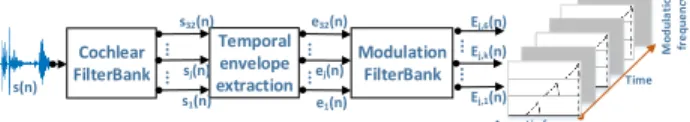
Many studies use a 2D convolution operation on a feature map and use RNN or LSTM on the segmented sub-sequence to get the speech signal relations. Mao et al. [17] trained an autoencoder followed by a CNN to learn salient feature maps from a spectrogram. Lim et al. [18] used deep CRNN to extract salient features by transforming the speech signal to 2D representations using short time Fourier transform (STFT). Keren et al. [19] and Neumann et al. [20] presented CNN in combination with LSTM to improve the recognition rate based on log Mel filter-banks. Recently, end-to-end SER from raw waveform is a new research direction based on significant ST feature learning abilities of neural networks. Trigeorgis et al. [21] used a 1D convolutional operation on the discrete-time waveform to predict dimensional emotions. However, the raw waveform is processed by an auditory system forming 4D representations rather than 1D or 2D forms. Moreover, the aforementioned Wu et al. [11] and Zhu et al. [12] just extracted modulation spectral features including centroid, skewness, kurtosis, and other statistical features from a modulation spectrum for emotion recognition but did not consider the richer original information. Cochlear FilterBank Temporal envelope extraction Modulation FilterBank s(n) s1(n) s32(n) e1(n) e32(n) Ej,1(n) sj(n) ej(n) Ej,6(n) ... ... ... ... ... Time Acoustic frequency M od ul a ti on fr e q u e n cy Ej,k(n) ...

Fig. 1. Signal processing steps to extract spectral-temporal representation

This paper proposes an end-to-end utterance-level emotion recognition system using a 3D-CRNN based on temporal modulation cues. This method firstly extracts temporal modulation cues via a cochlear filter and temporal envelope extraction of each filter. These cues contain ST integration representations directly as the 3D-CRNN input. The originality of this paper is that it is the first attempt to put temporal modulation cues in speech into the CNN simultaneously to extract high-level ST representation and is the first attempt to use 3D-CRNN to recognize speech emotions from raw data.

2. SPECTRAL-TEMPORAL REPRESENTATIONS 2.1. Overview of spectral-temporal representations

The ST representations are extracted using the signal processing steps depicted in Fig. 1. First, the emotional speech signal s(n) is filtered by a bank of 32 critical-band Gammachirp filters to emulate the processing performed by the cochlea (see Eq. (1)).

𝑠𝑗(𝑛) = ℎ𝑗(𝑛) ∗ 𝑠(𝑛) (1)

Where hj(n) is the impulse response of the jth channel and n is the sample number in the time domain. Second, the temporal envelope is extracted using the Hilbert transform or HWR to calculate the instantaneous amplitude ej(n) of the jth channel signal. Furthermore, the modulation filterbank is used for the kth sub channel in the jth channel signal to extract the ST modulation signal Ej,k(n). Eventually, 4D ST representations are obtained.

2.2. Cochlear filterbank

Gammachirp and Gammatone filterbanks as typical cochlear filterbanks model the basilar membrane motion well. Compared to the Gammatone filter, the Gammachirp filter is an asymmetric and nonlinear filter that has a similar shape to that of the cochlear filter [7]. Hence, the Gammachirp filter is used in this study. The impulse response of a Gammachirp filter is the product of the Gamma distribution and the sinusoidal tone. The bandwidth of each filter is described by an ERB, which is a psychoacoustic measure of the width of the auditory filter at each point along the cochlea.

gt(𝑡) = A𝑡𝑁−1_{exp(−2π𝑏}

𝑓ERB(𝑓0)𝑡) cos(2𝜋𝑓0𝑡 + 𝑐𝑙𝑛(𝑡) + φ) (2)

As shown in Eq. (2), where A, 𝑏𝑓, and N are parameters,

and A𝑡𝑁−1_{exp (−2π𝑏}

𝑓ERB(𝑓0)𝑡) is the amplitude term

represented by the Gamma distribution, 𝑓0 is the center

frequency of the filter, the cln(t) term is the monotonic frequency modulation term, φ is the original phase, and ERB(𝑓0) is an equivalent rectangular bandwidth in 𝑓0(𝑡) .

When c = 0, the chirp term, cln (t), vanishes, and this equation represents the complex impulse response of the Gammatone. Accordingly, the Gammachirp is an extension of the Gammatone with a frequency modulation term.

A m p lit ude A m p lit ude A m p lit ude A m p lit ude Anger _Happiness

Neutral Emotion Sadness

Fig. 2. Time-averaged modulation representation of sounds

2.3. Temporal Envelope Extraction

The temporal envelope is extracted using the Hilbert transform or HWR to simulate the functionality of the IHC. The half-wave or full-wave rectification produces distorted frequency components in the modulation domain, whereas the Hilbert transform provides a clear separation between the signal’s temporal envelope and fine structure. Hence, the Hilbert transform is used for temporal envelope extraction in this study.

2.4. Modulation filterbank

A modulation filterbank is used to extract the ST modulation representations over the joint acoustic-modulation frequency plane. By incorporating the cochlear filterbank and the modulation filterbank, a richer 4D ST representation is formed and used to analyze spectral and temporal relations. Figure 2 shows the modulation representation for the four emotions with a time-averaged pattern, where each one shown is the average over all the time frames for an emotion. “AFC” and “MFC” denote the acoustic and modulation frequency channels, respectively.

Such representations show that the energy of human vocal sound is mostly concentrated at 10 to 15 acoustic frequency channel for anger and happiness and at 5 to 12 acoustic frequency channel for neutral emotion and sadness. The energy is mostly concentrated at the lower modulation frequency channel with a peak at 4 Hz for neutral emotion. The peak shifts to a higher modulation frequency for anger and happiness, suggesting a faster speaking rate for these emotions. Happiness, however, shows a more abundant energy distribution in higher acoustic channels compared to anger’s energy distribution. In contrast to anger and happiness, neutral emotion, and sadness exhibit lower modulation frequency more prominently, suggesting lower speaking rates. The neutral emotion, however, also exhibits a prominent energy distribution in higher acoustic channels between 20 and 25. Sadness exhibits a discriminative energy distribution in the lower acoustic frequency channels over all modulation frequency channels.

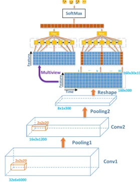
32x6x6000 2x2x20 16x3x1200 2x2x20 8x1x300 160x300 160x30x10 1 ... k ... 30 Conv1 Conv2 Pooling1 Pooling2 Reshape Fe at u re Time h h h h Max SoftMax h h ... h h h h Max h h ... Multiview Fe at u re

Fig. 3. Overview of 3D-CRNN model

This shows that different emotions have discriminative ST modulation representations, which are suitable to extract high-level ST representations for convolutional networks.

3. 3D CONVOLUTIONAL RECURRENT NEURAL NETWORKS

3.1. 3D-CRNN model

Inspired from biological neural networks, shadow or deep artificial neural networks were designed to extract features. CNNs can extract high-level multiscale ST representations using different receptive fields. RNNs can handle long-range temporal dependencies. For processing audio signals, CNNs/RNNs are used to achieve the function of the primary auditory cortex.

We put forward a 3D-CRNN model combining a CNN and RNN for emotion recognition from speech. Figure 3 shows the overview of the proposed methods. First, we feed the ST representations into the 3D CNN to learn high-level multiscale ST representations straightforwardly for a sequence of varied length. Nevertheless, LSTM/RNN is more suitable to learn the temporal information.

Table 1. 3D-CRNN architecture

Layer Input size Output size Kernel Stride

Conv1 32x6x6000 32x6x1200 2x2x20 1x1x5 Pool1 32x6x1200 16x3x1200 2x2x1 2x2x1 Conv2 16x3x1200 16x3x600 2x2x20 1x1x2 Pool2 16x3x600 8x1x300 2x3x2 2x3x2 RNN1 10x30x160 30x128 - - RNN2 30x128 128 - - MV 128 3x128 - - FC 3x128 4 - -

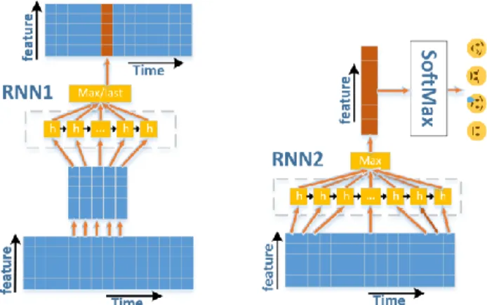
Fig. 4. First (left) and second (right) recurrent layers

Eventually, fully connected features are generally used as the LSTM input, but keeping the spatial correlation information in LSTM processes enables more informative ST representations to be learnt.

3.2. 3D convolutional layer

The 3D-CRNN architecture is described in Table 1. The first convolutional layer (Conv1) is used to extract 3D features that are composed of acoustic frequency, modulation frequency, and short-time windows. These features are another time sequence, which is the input of the second convolutional layer (Conv2) that models ST representations. The data format of the input and output data is reported as "DxHxW", where D, H, and W are the data in the acoustic frequency channels (depth), modulation frequency channels

(height), and time sequence (width), respectively.

Specifically, the input size is 32x6x6000. Additionally, the shape of the kernels is [2, 2, 20] in the conv1 and conv2 layers following the max-pooling operation. Finally, we get the output of pool2 with the shape of 8x1x300 and then reshape it to 2D shapes. The batch size and convolution filter size are equal to 20. Batch normalization is used before each convolutional layer. Experiments in this study also demonstrate that there will be a substantial speedup in training when using batch normalization.

3.3. Recurrent layer

We also use two recurrent layers to obtain different scale dependencies using the first recurrent layer (RNN1) for relatively short-term dependencies and the second recurrent layer (RNN2) for utterance-level dependencies.

Figure 4 shows the first and second recurrent layer. For RNN1, the input of the layer is 300x160, representing the time sequence length and feature size, respectively. The time sequence is divided into 30 windows, and each window includes 10 time frames. The time sequence is fed frame by frame into the first recurrent layer. Then, the hidden states of the recurrent layer along the different frames of the window are used to compute the extracted features [19].

Fig. 5. Comparison of recognition accuracy of different models on IEMOCAP database

The output of this layer for each window is the cell state vector of the last time frame in each window. For each window, each layer extracts 128 features. Finally, we create a new sequence with a length of 30x128 to put into RNN2. For RNN2, the whole sequence is fed into the LSTM model, and max-pooling is used to generate 128 feature sequences. After applying max-pooling, the resulting sequence contains temporal features of the sequence and can be fed into the fully connected layer for classifying.

3.4. Multi-view learning

For RNN1, 30 time windows are obtained, and each time window includes 10 time frames. Moreover, we utilize multi-view learning to obtain more information. In this study, we just use unidirectional LSTM because of the varied length for each utterance in the database. For obtaining more dependency information, we shift the time sequence twice, and each shift is equal to 3 and 6, respectively. Finally, we feed this shifted time sequence into RNN2 as a new sequence.

4. EXPERIMENT RESULTS 4.1. Experimental database of emotional speech

For our experiments, we used the interactive emotional dyadic motion capture (IEMOCAP) database [22], which is a well-known dataset for speech emotion recognition comprising of scripted and improvised multimodal interactions of dyadic sessions. The dataset consists of around 12 hours of speech from 10 human subjects and is labeled by three annotators for emotions such as happy, sad, angry, excited, and neutral, along with dimensional labels such as valence and arousal. All recordings have the structure of a dialogue between a man and a woman either scripted or improvised on the given topic. For this study, we merged happy and excited into one class: happy. We took 5,531 utterances for all sessions. The mean length of all the turns is 4.55 s (max.: 34.14 s, min.: 0.58 s). Since the input length for a CNN has to be equal for all samples, we set the maximal length to 7.5 s (mean duration plus standard deviation). Longer turns were cut at 7.5 s, and shorter ones were padded with zeros.

Table 2. Setup for modulation spectral features Name Value Sampling frequency 16000 Hz Modulation filterbank sampling frequency 800 Hz Gammachirp channels 32 Modulation sub-channel 6

Sound pressure level 60 dB

4.2. Setup for modulation spectral features

We first applied a pre-emphasis filter to the signal to amplify the high frequencies to compensate for the energy loss in the outer-middle ear and then used normalization to remove the difference of the speakers by mapping the values of signals to mean 0 and the standard derivation to 1.

Furthermore, we introduced the compressive

Gammachirp filterbank to accommodate the compressive characteristics. To get the data from the Gammachirp filterbank, the frequency distributed on the ERB scales was between 100 Hz and 8 kHz. The modulation filterbank was also used to control the envelopes of octave bands from 2 to 64 Hz, consisting of one low-pass filter and five band-pass filters. The detailed setup is shown in Table 2.

4.3. Hyper parameters for 3D-CRNN

For all random weight initializations, we chose L2 regularization. The parameters were learned in an end-to-end manner, meaning that all parameters of the model were optimized simultaneously using the Adam optimization method with a learning rate of 1e-4 to minimize the chances of having a cross-entropy objective. Moreover, we used a rectified linear unit (ReLU) as the activation function, which brought the non-linearity into the networks. To avoid overfitting when training our networks, we used a dropout rate of 0.5 after the second recurrent layer.

4.4. Comparison Experiments

There were three comparison experiments named 3D CNN, 3D CLSTM, and 3D CRNN-sv. All these models had the same layers from conv1 to pool2 with the shape of 300x160.

3D CNN: Adding two extra 2D convolutional layers and pooling layer (with 2x2 kernel and 2x2 stride) onto the top of pool2, and then was followed by a fully connected layer.

Table 3. Comparison of proposed method and other methods on IEMOCAP database Method WA UA Year Ref [23] 54.3% 48.2% 2014 Ref [25] 48.1% 49.09% 2016 Ref [24] 54% 54% 2017 Ref [20] 56.1% - 2017 Our work 61.98% 60.93%

3D CLSTM: Similar to the 3D-CRNN model except without the RNN1 and MV layer. For RNN2, the whole sequence with the shape of 300x160 was fed into the LSTM model, and max-pooling was used to generate 128 feature sequences.

3D CRNN-sv: This was a single-view way for the 3D-CRNN model. Similar to the 3D-3D-CRNN model except without the MV layer. The output size of FC was 128.

4.5. Experiments results

To train the models in a speaker-independent manner, we used leave-one-session-out cross-validation. We used utterances from eight speakers to construct the training datasets and used the other two speakers for the test.

We used two measures to evaluate the performance: weighted accuracy (WA) and unweighted accuracy (UA). WA is the classification accuracy of the entire test data set, and UA is the average of the classification accuracy for each emotion. The results obtained for each method are shown in Fig. 5. They show that the 3D-CRNN with multi-view results in better recognition accuracy with 61.98% and 60.93% in WA and UA measures. This shows that more multiscale information was obtained from the multi-view model. The results also show that the 3D CNN had poorer accuracy than that of the other models because of the absence of a recurrent layer. This also demonstrates the importance of the sequential dependencies information for emotion recognition from speech.

Table 3 shows that the proposed method outperformed the other methods. Han et al. [23] firstly extracted the segment-level emotion state distributions utilizing the features (F0 and MFCC) based on the DNN model and used an extreme learning machine (ELM) to identify utterance-level emotions. Chernykh et al. [24] proposed a CTC approach based on RNN to recognize the utterance-level emotions utilizing MFCC and spectrum properties like flux and roll-off features. The method of Ghosh et al. [25] learns utterance specific representations by a combination of stacked autoencoders and bidirectional LSTM trained on 128 bin FFT spectrograms. Overall, the proposed approaches significantly outperform the previous best accuracy result with 5.88% (from 56.1% to 61.98%) and 6.93% (from 54% to 60.93%) absolute accuracy improvement in WA and UA measures, respectively.

5. CONCLUSION

In this paper, we studied auditory-inspired end-to-end recognition of emotional speech using a 3D-CRNN model based on temporal modulation cues. Convolutional networks can reconstruct multiscale ST representations, and recurrent networks can obtain the long-term dependencies for emotion recognition. The experimental results demonstrate that our method is an effective way to design an emotion recognition system by mimicking the human auditory system. In the

future, we will compare Gammachirp and the Gammatone filter with a different number of acoustic and modulation channels. Furthermore, we will try to extract fundamental frequency information along with the ST features using multitask learning.

6. ACKNOWLEDGEMENTS

This study is supported by JAIST research grants. The study is supported partially by JSPS KAKENHI Grant (16K00297).

7. REFERENCES

[1] S. G. Koolagudi and K. Rao, “Emotion recognition from speech: a review,” International journal of speech technology, 15.2 (2012): 99-117.

[2] T. Dau, B. Kollmeier, and A. Kohlrausch, “Modeling auditory processing of amplitude modulation. I. Detection and masking with narrow-band carriers,” Journal of the Acoustical Society

of America, 1997, 102(5): 2892-2905.

[3] A. R. Møller, “Unit responses of the rat cochlear nucleus to tones of rapidly varying frequency and amplitude,” Acta

Physiologica, 1971, 81(4): 540-556.

[4] N. Suga, “Analysis of information-bearing elements in complex sounds by auditory neurons of bats,” Audiology, 1972, vol. 11, pp. 58–72.

[5] T. Chi, P. Ru, and S. A. Shamma, “Multiresolution spectrotemporal analysis of complex sounds,” The Journal of

the Acoustical Society of America, 2005, 118(2): 887-906.

[6] R. F. Lyon, “A computational model of filtering, detection, and compression in the cochlea,” in Proceedings of IEEE ICASSP, 1982, pp. 1282-1285.

[7] T. Irino and R. D. Patterson, “A dynamic compressive gammachirp auditory filterbank,” IEEE/ACM Transactions on

Audio, Speech, and Language Processing,14(6), pp. 2222–

2232, Nov. 2006.

[8] R. D. Patterson, M. H. Allerhand, and C. Giguere, “Time‐ domain modeling of peripheral auditory processing: A modular architecture and a software platform,” The Journal of the

Acoustical Society of America, 98.4 (1995): 1890-1894.

[9] M. Unoki, T. Irino, and R. D. Patterson, “Improvement of an IIR asymmetric compensation gammachirp filter,” Acoustical

Science and Technology, 22.6 (2001): 426-430.

[10] N. Moritz and B. Kollmeier, “An auditory inspired amplitude modulation filter bank for robust feature extraction in automatic speech recognition,” IEEE/ACM Transactions on

Audio, Speech, and Language Processing, 23.11 (2015):

1926-1937

[11] S. Wu, T. H. Falk, and W. Y. Chan, “Automatic speech emotion recognition using modulation spectral features,”

Speech communication, 2011, vol. 53, no. 5, pp. 768-785.

[12] Z. Zhu, R. Miyauchi, Y. Araki, and M. Unoki, “Modulation Spectral Features for Predicting Vocal Emotion Recognition by Simulated Cochlear Implants,” in Proceedings of interspeech, 2016, pp. 262-266.

[13] J. H. Mcdermott, E. P. Simoncelli, “Sound texture perception via statistics of the auditory periphery: evidence from sound synthesis,” Neuron 71.5(2011):926-940.

[14] Y. LeCun and Y. Bengio, “Convolutional networks for images, speech, and time series,” The handbook of brain theory and

neural networks, 1995, p. 3361.10.

[15] F. E. Theunissen, K. Sen, and A. J. Doupe, “Spectral-temporal receptive fields of nonlinear auditory neurons obtained using natural sounds,” Journal of Neuroscience, 20.6 (2000): 2315-2331

[16] S. Hochreiter and J. Schmidhuber. “Long short-term memory,”

Neural computation, 1997, 9(8): 1735-1780.

[17] Q. Mao, M. Dong, Z. Huang, and Y. Zhan, “Learning salient features for speech emotion recognition using- convolutional neural networks,” IEEE Transactions on Multimedia, vol. 16, no. 8, pp. 2203-2213, 2014.

[18] W. Lim, D. Jang, and T. Lee, “Speech emotion recognition using convolutional and Recurrent Neural Networks,” in

Proceedings of APSIPA, 2016, pp. 1-4.

[19] G. Keren and B. Schuller, “Convolutional RNN: an enhanced model for extracting features from sequential data,” in

Proceedings of IJCNN, 2016, pp. 3412-3419.

[20] M. Neumann and Vu, N. T, “Attentive Convolutional Neural Network based Speech Emotion Recognition: A Study on the Impact of Input Features, Signal Length, and Acted Speech,”

arXiv preprint arXiv:1706.00612, 2017.

[21] G. Trigeorgis, F. Ringeval, R. Brueckner, e E. Marchi, M. A. Nicolaou, B. Schuller, and S. Zafeiriou, “Adieu features? end-to-end speech emotion recognition using a deep convolutional recurrent network,” in Proceedings of IEEE ICASSP, 2016, pp. 5200-5204.

[22] C. Busso, M. Bulut, C. Lee, and A. Kazemzadeh. “IEMOCAP: Interactive emotional dyadic motion capture database,”

Language resources and evaluation, 2008, pp: 335-359.

[23] K. Han, D. Yu, and I. Tashev, “Speech emotion recognition using deep neural network and extreme learning machine,” in

Proceedings of interspeech, 2014, pp. 223-227.

[24] V. Chernykh, G. Sterling, and P. Prihodko, “Emotion Recognition From Speech With Recurrent Neural Networks,”

arXiv preprint arXiv:1701.08071, 2017.

[25] S. Ghosh, E. Laksana, L. P. Morency, and S. Scherer, “Learning representations of affect from speech,” arXiv