How to Optimally Measure a Momentum on a Half Line in Quantum Mechanics (Non-Commutative Analysis and Micro-Macro Duality)

How to

Optimally Measure

a Momentum on a

Half Line

in Quantum

Mechanics

1

Yutaka Shikano and

Akio

Hosoya

Department of Physics,

Tokyo Institute of Technology

Abstract

We cannot perform the projective measurement of a momentum on a half line

since it is not an observable. Nevertheless, we would like to obtain some physical

information of the momentum on a half line. We define an optimality for

mea-surement as minimizing thevariance between an inferred outcome ofthe measured system beforea measuringprocess anda measurementoutcome ofthe probesystem

after themeasuring process, restricting our attention to the covariant measurement

studied by Holevo. Extending the domain of the momentum operator on ahalf line by introducing a two dimensional Hilbert space to be tensored, we make it self-adjoint and explicitly construct a model Hamiltonian for the measured and probe

systems. By taking the partial trace over the newly introduced Hilbert space, the

optimal covariant positive operator valued measure (POVM) ofa momentum on a

half line is reproduced. We physically describe the measuring process to optimally evaluate the momentum ofa particle on a half line.

1

Introduction

Quantum theory begins in 1899 with the discovery of the Planck law in black body

radiation. Its formulation

was

initiated by Heisenberg and Schr\"odinger respectively. In

1932,

von

Neumann

mathematically

formulated

quantum mechanics [2]

as

the following

postulates.

Postulate 1 (Representations of states and observables). $\mathcal{A}ny$ quantum system $S$ is

as-sociated with

a

separable Hilbert space $\mathcal{H}_{S}$, called the state space

of

S. $\mathcal{A}ny$ quantum state

of

$S$ is the element $|\psi\rangle$

of

the Hilbert space and is represented in one-to-one

correspon-dence by

a

positive operator $\rho=|\psi\rangle\langle\psi|$ with unit trace, called

a

density opemtor. $\mathcal{A}ny$

observable

_of

$S$ is represented in one-to-one correspondence by

a

self-adjoint operator $A$

densely

_defined

on

$\mathcal{H}_{S}$.

Postulate 2 (Schr\"odinger equation).

_If

$S$ is isolated in a time interval $(t, t’)$, there is a

unitary operator $U$ such that

if

$S$ is in

$\rho$ at $t$ then $S$ is in $\rho=U\rho U^{\uparrow}at$ $t’$.

Postulate 3 (Born formula). Any observable $A$ takes the value in

a

Borel

set

$\Delta$ in any

$\rho$

with the probabilityTr$[E^{A}(\Delta)\rho]$, where $E^{A}(\Delta)$ is thespectral projection

of

A corresponding

to $\Delta$.

Postulate 4 (Composition rule). The composite system $S+S’$ is the tensor product

$\mathcal{H}_{S}\otimes \mathcal{H}_{S^{t}}$

of

their state spaces.

lThis proceeding is for the talk at RIMS Research Meeting ”Micro-Macro Duality in Quantum

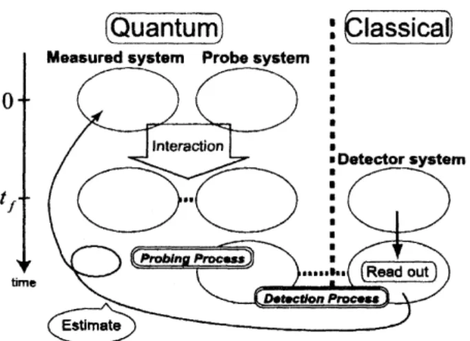
Figure 1:

Scheme

of measuring processes.

We switch

on

the interaction between the

measured

and probe systems in the first step to obtain the measurement outcome ofthe

probe system in the secondstep. We infer the observable of the measured system

at

$t=0$

from the outcome of the probe system at $t=t_{f}$ in the third step.

Whilehe discussedmeasuringprocesses, he failed togivethe mathematicalpostulateof

measurement. Thereafter

Ozawa

introducedthe postulate ofmeasurement [3] toconsider

the measured system and probe system.

Postulate 5 (Representation of generalized measurement). When any observable $A$

of

the measured system is measured in any state $\rho_{sys}$

before

measurement,

we

obtain that the

state

_after

measurement is $M(\Delta)\rho_{sys}=\ulcorner fr_{en\tau},[U(\rho_{sv^{g}}\otimes\rho_{prob})U^{\uparrow}]$ and $A$ takes the value in

a

Borel set $\Delta$ with the probability _{$Tr_{sys}[\rho_{sys}M(\Delta)]$}, where the time evolution opemtor is

defined

on

the composite system $\mathcal{H}_{sys}\otimes \mathcal{H}_{prob}$.

$M(\Delta)$ is often

called

positive operatorvalued

measure

(POVM)

or

completely positive

tracepreserving (CPTP) map of measurement. The concept ofmeasurement is illustrated

in Fig. 1.

So

measurement is represented by a

POVM

while

an

interaction between

a

measured and probe system is not known. To consider

an

experimental setup of

measure-ment,

we

need to knowthe interaction. We

now

derive the measurement interaction from

a given POVM under

a

specific condition about measurement of a momentum

on

a half

line.

For measuring processes,

we

shall consider

an

optimal measurement initiated by

Hel-strom $[$4]. He

defined

an

optimality of

a

measuring process to minimize the variance

between

an

outcome of a measured system

_before

the interaction and

a

measurement

out-come

of

a

probe system

_after

the interaction. The optimal measurement sets upper limits

to

a

POVM. In thispaper,

we

explicitly constmct amodel Hamiltonian whichreproduces

the optimal POVM in a special case, while a general method is not available to construct

a

measurement

model

from

a

given

POVM.

This paper has two main results. One is to explicitly construct

an

optimal covariant

measurement model Hamiltonian to

measure

a momentum of

a

particle. In

case

of

a

whole line, optimal covariant measurement corresponds to projective measurement, that

half line system using the optimal covariant measurement model. Throughout this paper,

we

take the unit $\hslash=1$.

2

Review

of Optimal

Covariant Measurement

Let

us

consider

a

measuring process described by

an

interaction between

a

measured

system and a probe system,

the

latter of which is the part of the measuring apparatus

as

a

whole. To establish the relationship between the measured and probe systems,

we

consider the momentum space $\Omega=\mathbb{R}$ and a projective unitary representation ofthe shift

group

of$\Omega$. Stonc’s theorem tells

us

that the unitary representation is given by

$parrow V_{p}=e^{-i\rho\hat{x}}$, (1)

where

$\hat{x}$ is

the

position operator.

Definition 1. A

POVM

$M(dp)$ is covanant vnth respect to the representation $parrow V_{p}$

if

$V_{p}^{\dagger}M(\Delta)V_{p}=M(\Delta_{-p})$, $p\in\Omega$ (2)

for

any

$\Delta\in \mathcal{A}(\Omega)$, where

$\Delta_{p}=\{p’|p’=p+p’’, p’’\in\Delta\}$ (3)

is the image

_of

the set $\Delta$ under the

transformation

$p$ and$\mathcal{A}(\Omega)$ is the Borel $\sigma- field$

of

$\Omega$.

The covariant POVM has the property in the following form by using the Bom

for-mula [2, 9], $Pr\{\hat{p}\in\Delta_{p}\Vert\rho_{p+p_{0}’}\}=Tr\rho_{p+p_{0}’}M(\Delta_{p})$ $=TrV_{-p}\rho_{p_{0}’}V_{-\rho}^{\dagger}M(\Delta_{p})$ $=T\}\rho_{p_{0}’}V_{p}^{\underline{\dagger}}M(\Delta_{p})V_{-p}$ $=Tr\rho_{p_{0}’}M(\Delta)$ $=Pr\{\hat{p}\in\Delta\Vert\rho_{p_{0}’}\}$. (4)

That is, when the measured system is arbitrarily shifted, the measurement outcome is

shifted by the

same

amount. This idealized measurement is called a covanant

measure-ment. The curious point is to correspond to the opitmal POVM under an unbiased

condition by Hayashi and Sakaguchi [5] and

more

realistic measuring device is subject to

an

unbiased condition only locally

as

discussed by

Hotta

and

Ozawa

[6].

By

von Neumann’s

spectral theorem, any Hilbert

space

$\mathcal{H}$

can

be formally described

as

the direct integral of

a

Hilbert

space

$\mathcal{H}_{x}$,

$\mathcal{H}=\int\oplus \mathcal{H}_{x}dx$, (5)

so

that any state vector $\psi\in \mathcal{H}$ is described by the vector-valued function $\psi=[\psi_{x}]$ with

$\psi_{x}\in \mathcal{H}_{x}$ introducing a convenient notation $[\cdot][7,9]$. There, a position operator $\hat{x}$ acts

as

multiplication operators

in this notation. The

same

notation $[\cdot]$ is used for

an

operator-valued function. A kernel $[K(x, x’)]$_{, where} $K(x, x’)$ _{is a mappingfrom} $\mathcal{H}_{x’}$ to $\mathcal{H}_{x}$ for all$x$ and $x’$, defines an operator

$\hat{K}$ on

$\mathcal{H}$. We can write

$\hat{K}\psi=[K(x, x^{l})][\psi_{x’}]=[\int K(x, x’)\psi_{x’}dx’]$ . (7)

The equation (6) and (7)

can

be rephrased by the bracket notation

as

$\hat{x}|\psi\rangle=\int dx|x)x\langle x|\psi)$, (8)

$\hat{K}|\psi\rangle=/dx/dx’|x\rangle K(x, x’)\langle x’|\psi\rangle$, (9)

respectively. Also

we

express the

norm

in $\mathcal{H}_{x}$

as

1

$\Vert_{x}$

.

We are now

in

a

position to explicitly describe the covariant

POVM

as

follows.

Theorem 1 (Holevo [7]). Any covamant POVMin $\mathcal{H}$ has the

form

$M(dp)=[K(x, x’)e^{i(x-x’)p} \frac{dp}{2\pi}]$ , (10) $\prime inh_{l}ere[K(x, x’)]$ is apositive

definite

kernel satisfying $K(x,x)\equiv I_{x}$, the identity mapping

from

$\mathcal{H}_{x}$ to

itself.

In the above discussion,

we

have assumed that system and probe observables

are

isometric to obtain (10)

as

the

POVM.

The proof of

Theorem

1 is given in Appendix A

of $[1|$.

Next

we

tum to

a

measuring process. First,

we

couple

a

measured system to

a

probe

system. Second, the combined system is evolved in time. Finally,

we

measure

the probe

observable. The sequence of processes enables

us

to retrospectively evaluate the system

observable at the starting time by the measurement outcome of the probe observable at

the end time (See Fig. 1).

So we

define the optimal covariant measurement

as

an

optimal

evaluation of the syst$em$ observable by the outcome ofthe probe observable.

Let us

assume

that $W(p-P)$ is

a

deviation function, which expresses the variance

between the inferred “measurement” outcom$ep$ of the system momentum before the

interaction and the measurement outcome $P$ofthe probe momentumafter the interaction,

satisfying

$W(p)=-/e^{ipx}\tilde{W}(dx)$, (11)

for

an

even

finite

measure

$\tilde{W}(dx)$

on

$\mathbb{R}$. Let

us

consider the condition

to

minimize the

variance

$R_{\rho} \{\Lambda I\}=\int_{\Omega}W(p-P)\mu_{\rho}(dp)$, (12)

where $\mu_{\rho}(dp)\equiv$ Tlr$\rho M(dp)$ is the probability distribution for the pure state $\rho=|\psi\rangle\langle\psi|$.

Because of covariance,

we

rewrite (12)

as

$R_{0}\{M\}=/\Omega^{W(p)\mu_{\rho 0}(dp)}$

where

$\Phi_{\rho}(x)\equiv/\iota^{e^{ixp}\langle\psi|M(dp)\psi\rangle}$ (14)

is

a

characteristic function of $\mu_{\rho}(dp)$. We get from Eq. (10)

$\Phi_{\rho}(x)=/\langle\psi_{\mu}|K(\mu, \mu-x)\psi_{\mu-x}\rangle d\mu$. (15)

Since the integral

converges

by the Cauchy-Swartz inequality and the condition $K(x, x)=$

$I_{x}$, $Re\Phi_{\rho}(x)\leq\Phi_{*}(x)\equiv/\Vert\psi_{\mu}\Vert_{\mu}\Vert\psi_{\mu-x}\Vert_{\mu-x}d\mu$, (16)

so

that $R_{0} \{M\}\geq-/\int\Vert\psi_{\mu}\Vert_{\mu}\Vert\psi_{\mu-x}\Vert_{\mu-x}d\mu\tilde{W}(dx)$ $\equiv R_{0}\{M_{0}\}$, (17) where $M_{0}(dp)=[ \frac{\psi_{x}\cdot\psi_{x}^{\dagger}}{\Vert\psi_{x}||_{x}\Vert\psi_{x}’,\Vert_{x’}}e^{i(x-x’)p}\frac{dp}{2\pi}]$, (18)

by transforming $\mu-x$ to $x^{l}$. Note that Eq. (18) does not depend

on

the choice of the

deviation function $W(p-P)$ because of the covariance. In the

case

of the whole line

system, the optimal covariant

POVM

(18) in the bracket notation

expresses

$M_{0}(dp)= \int_{R}dx\int_{R}dx’|x)e^{i(x-x’)p}\frac{dp}{2\pi}\langle x’|$, (19)

noting that the normalized term $\frac{\psi_{x}\psi^{t},}{\Vert\psi_{x}\Vert_{x}||\psi_{x},\Vert_{x}}$ is the identity in the bracket notation. Using

the Fourier transformation,

$|p \rangle=\frac{1}{\sqrt{2\pi}}/\mathbb{R}^{dxe^{ipx}|x\rangle}$

’ (20)

Eq. (19) is transformed to the following equation,

$M_{0}(dp)=|p\rangle\langle p|dp$, (21)

to obtain the projective measurement of

a

momentum

on a

whole line. To summarize the

above discussion,

we

obtain the optimal covariant POVM (18) to minirnize the estimated

variance between the system and probe observables [7, 8]. We emphasize that Eq. (18)

remains valid

even

when

we

change the domain of $x$

.

3

Optimal

Measurement

Model

on a

Whole

Line

Intheprevious section,

we

haveobtained the optimal covariant POVM. We

are

now

going

to explicitly construct a Hamiltonian for

a

measurement model to realize the POVM.

the system observable for a given Hamiltonian of

a

combined system, it is not to find a

Hamiltonian from agiven POVM. In the two dimensional case, there is a way to construct

a

model

Hamiltonian

from

a

given POVM [11]. Once the Hamiltonian for the combined

system is found,

we

can

physically realize the given POVM in principle. In the infinite

dimensionalcase,

we

heuristically explore the optimal covariantPOVM for the momentum

in measuring processes in the following way. In this section, we preparatively discuss

measurement of the momentum of

a

particle

on a

whole line and then apply the results

to that

on

a half line

in the next section. To make

our

exposition shorter,

we

assume

that

the wave functions $\{\psi_{x}\}$

are

normalized and the

measure

$\frac{d}{2}R\pi$ is omitted in Eq. (18). Then

Eq. (18) is simply

$M_{0}=[\psi_{J_{x}}\cdot\psi_{x}^{\dagger},e^{i(x-x’)p}]$ . (22)

Let

us

consider

a

model

Hamiltonian[12],

$\hat{\mathcal{H}}_{c,om}=\frac{1}{2m}\hat{p}^{2}+\frac{1}{2M}\hat{P}^{2}+g\hat{P}\hat{x}\delta(t)+\frac{m\omega^{2}}{2}\hat{x}^{2}$

$\equiv\hat{\mathcal{H}}_{0}+g\hat{P}\hat{x}\delta(t)$, (23)

where

a

pair $(\hat{x},\hat{p})$

are

the position and thc momentum operators of the measured

sys-tem,

a

pair $(\hat{X},\hat{P})$

are

those of the probe system and $\delta(t)$ is the Dirac $\delta$-function. This

Hamiltonian

is modeled from the following consideration. We take the potential of the

measured system

as a

harmonic oscillator for simplicity and the probe system is assumed

to be a free particle system. Furthermore, the interaction is assumed to be instantaneous

with

a

coupling constant $g$. The interaction term $g\hat{x}\hat{P}\delta(t)$ is chosen by the following

rea-soning. Because of the covariance, i.e., the measurement value $\tilde{P}$

of the probe observable

corresponds to the “_{measurement” value}

$\tilde{p}$ ofthe system observable at

a

certain time, we

are

led to

an

interaction of the momentum $\hat{P}$ of the probe system. Since the exponents

in the optimal covariant POVM (22) has a quadratic form, a possible interaction term is

either $g\hat{x}\hat{P}$

or

$g\hat{p}\hat{P}$. The latter is excluded because it does not influence the momentum

of the measured system.

Let

us

assume

that the measured system itself is weakly coupled to

a

bulk system at

zero

temperature.

We

consider the measuring

process

from the time $t=0-$ to $t=t_{f}$.

Fkom Eq. (23) the evolution operator $\hat{U}$ becomes

$\hat{U}=$ Texp _{$(-i \int_{0-}^{t_{f}}\hat{\mathcal{H}}_{com}dt)$}

$=$ Texp $(-i/\epsilon t_{f}\hat{\mathcal{H}}_{0}dt)\exp(-i/-\epsilon\epsilon g\hat{P}\hat{x}\delta(t)dt)$

$=T$ cxp $(-il^{t_{f}}\hat{\mathcal{H}}_{0}dl)$ cxp $(-ig\hat{P}\hat{x}(0))$ , (24)

where $\epsilon$ is an infinitesimal positive parameter and $T$ stands for the time-ordered product.

We construct the Kraus operator$[\hat{\mathcal{A}}_{xx’}]$ from the evolution operator

as

follows. Given

the initial probe stat$e|\tilde{P}\rangle$,

an

eigenstat_$e$ of the momentum $\hat{P}$ ofthe

Figure 2: An optimal covariant measurement model. By the instantaneous interaction

between the measured and probe systems, the measured system is entangled with the

probe system.

On

the other hand, the measured system is coupled with the bulk system

at

zero

temperature to dissipate the

energy

of the

measured

system. Thus

we

optimally

evaluate the system observable at $t=0$ inferred from the outcome of the probe system

at $t=\infty$ by the momentum conservation law.

that

$\hat{A}_{xx’}=/\langle P|\langle x|\hat{U}|x’\rangle|\tilde{P}\rangle dP$

$= \sum_{j}\langle x|$Texp

$(-i \int_{\epsilon}^{t_{f}}\hat{\mathcal{H}}_{0}dt)|j\rangle\psi_{x,j}^{\dagger}\exp(-ig\tilde{P}x(0))$

$arrow\psi_{x}\cdot\psi_{x}^{\dagger},$_{$\exp(-ig\tilde{P}x(0))$}

a

_{$s$ $t_{f}arrow\infty$}, (25)

where $|P\rangle$ is

an

eigenstate of $\hat{P},$

$\psi_{x_{2}j}$ is

a wave

function corresponding to the j-th

energy

eigenstate $|j\rangle$ and $\psi=[\psi_{x}]$ is the ground state of the free Hamiltonian

$\hat{\mathcal{H}}_{0}$. In the last

line of (25), the ground state is pickcd up in the limit $t_{f}arrow\infty$, or physically speaking,

we

measure

the prob$e$ observable after sufficient time passes. $Re$call that the standard

$i\epsilon$ prescription [13] implicitly

assumes

that the measured system itself is weakly coupled

to the bulk system at

zero

temperature. The equation (25) is the matrix element of the

Kraus

operator $[\hat{\mathcal{A}}_{xx’}]$.

From

the Kraus operator,

we

calculate the

POVM as

$M=[ \int\hat{A}_{x’ x}^{\dagger},,A_{xx’’}dx^{l/}]=[\psi_{x}^{\dagger},$

.

$\psi_{J_{x}}\exp(-ig\tilde{P}\{x(0)-x’(0)\})]$ . (26)

We identify $g\tilde{P}$ with the measurement outcome $P$ itself ofthe probe observable to

repro-duce the optimal covariant POVM (22)

on a

whole line.

Now, we physically describe how

we

optimally infer the momentum of the measured

system just before the measuring process. First,

we

couple the measured system to the

probe syst$em$ instantaneously. Second,

we

keep the measured system in contact with the

bulk system at

zero

temperature and wait for a sufficiently long time. Since the

energy

of

the measured system is dissipated to the bulk system, the

state

of the

measured

system

$\omegaarrow 0$ of the interaction Hamiltonian (23), the momentum ofthe measured system_{$p_{sys,\infty}$}

becom

es zero

at $t_{f}=\infty$. Accordingto the momentum conservation law, we obtain

$p_{sy0}6,+p_{p,0}=p_{sys,\infty}+p_{p,\infty}=p_{p,\infty}$, (27)

where $p_{sys,t}$

and

$p_{p,t}$

are

the

momenta

of

the measured

system and the probe system at

a

time $t$.

Since we

can

control the probe system,

we

can

precisely infer the “measurement”

value $p_{9ys,0}$ ofthe momentum of the measured system at the beginning ofthe measuring

process from the measurement outcome $p_{p,\infty}$, which we

measure

in the probe system at

$t_{f}=\infty$ (See Fig. 2). If $\omega$ of the Hamiltonian (23)

were

finite, the variance of the

momentum of the measured system would remain finite due to the

zero

point oscillation

and Eq. (27) would be modified.

Although

we

have assumed that the potential of the

measured

system is given by

the harmonic oscillator, the potential could actually be any

convex

function since the $i\epsilon$

prescription picks up the ground state at $t_{f}arrow\infty$.

4

Quantum

Mechanics

on a

Half Line

According to the functional analysis,

on

which the mathematical foundation ofquantum

mechanics [2] is based,

an

operator $\hat{A}$ is symmetric if $\hat{\mathcal{A}}=\hat{A}\dagger$,

where $\hat{\mathcal{A}}\dagger$

is the Hermite

conjugate. Further,

a

symmetric operator $\hat{A}$

is self-adjoint if$\mathcal{D}(\hat{A})=\mathcal{D}(\hat{A}\dagger)$, where $\mathcal{D}(\hat{A})$

is the domain of the operator $\hat{A}_{-}$

In quantum mechanics, the observables

are

defined

as

self-adjoint operators, which have real spectra [14]. Symmetric operators, however, do

not necessarily have

a

real spectrum. We need to classify symmetric operators into

self-adjoint operators, essentially self-self-adjoint operators, self-self-adjoint extendable operators and

non-self-adjoint extendable operators (for the definitions,

see

the book [14]).

A

criterion

is known

as

the deficiency theorem (See Appendix A).

Let

us

specifically consider

a

quantum system

on a

half line $\mathbb{R}+\equiv[0, \infty)$

.

There

have been

many

works conceming this problem since the beginning of quantum

mechan-ics [15, 16, 17], e.g., the singular potential [18, 19, 20, 21]. Recently, Ful\"op et al. have

studied boundaryeffects [22, 23, 24] and Twamley and Milburn havediscussed

a

quantum

measurement model

on a

halfline by changing the coordinate $x\in \mathbb{R}_{+}$ to log$x\in \mathbb{R}[25|$.

In the following consideration, we characterize the half linc system as follows. Let

us

take a Hilbert space $\mathcal{H}_{+}\equiv \mathcal{L}^{2}(\mathbb{R}_{+})$ and

a

momentum operator$\hat{p}_{+}$ in $\mathcal{H}_{+}$ defined by

$\hat{p}_{+}\psi(x)=\frac{1}{i}\frac{d}{dx}\psi(x)$,

$\mathcal{D}(\hat{p}_{+})=\{\psi\in \mathcal{H}_{+};\psi(0)=0,$ $I_{0}^{\infty}| \frac{d}{dx}\psi(x)|^{2}dx<\infty\}$ (28)

Then we can see that $\hat{p}+$ is symmetric since

$\langle\phi|\hat{p}_{+}\psi\rangle=\frac{1}{i}/0\infty\overline{\phi(x)}\frac{d}{dx}\psi(x)dx$

$=[ \frac{1}{i}\overline{\phi(x)}\psi(x)]_{0}^{\infty}-\frac{1}{i}/0^{\infty}\frac{d}{dx}\overline{\phi(x)}\psi(x)dx$

$=/0^{\infty}\overline{\frac{1}{i}\frac{d}{dx}\phi(x)}\psi(x)dx$

$=\langle\hat{p}1\phi|\psi\rangle$, (29)

$\psi\in \mathcal{D}(\hat{p}_{+})$ $\phi\in \mathcal{D}(\hat{p}_{+}^{\dagger})$, (30)

where $\hat{p}_{+}^{\dagger}=\frac{1}{i}\frac{d}{dx}$ with

$\mathcal{D}(\hat{p}_{+}^{\dagger})=\{\psi\in \mathcal{H}_{+};\int_{0}^{\infty}|\frac{d}{dx}\psi(x)|^{2}dx<\infty\}$ . (31)

Therefore

we

conclude

that

$(\hat{p}_{+}, \mathcal{D}(\hat{p}_{+}))\subsetneq(\hat{p}_{+}^{\dagger}, \mathcal{D}(\hat{p}_{+}^{\dagger}))$ since $\mathcal{D}(\hat{p}_{+})\neq \mathcal{D}(\hat{p}_{+}^{\dagger})$

. So

the

momentum operator $\hat{p}+$ on a half line is symmetric but not self-adjoint, i.e., not

an

observable.

5

Optimal

Measurement

Model

on a

Half

Line

Let

us

apply the optimal measurement model to the half line system.

We

have already

seen that the momentum operator (28) is not self-adjoint. First,

we

extend the domain

of$\hat{p}+\acute{a}$ la Naimark

so

that the extended operator $\hat{p}$ is self-adjoint. The extended Hilbert

space is

$\mathcal{H}=\mathcal{H}_{+}\otimes \mathcal{H}_{2}$, (32)

where $\mathcal{H}\equiv \mathcal{L}^{2}(\mathbb{R}),$ $\mathcal{H}_{+}\equiv \mathcal{L}^{2}(\mathbb{R}_{+})$ and $\mathcal{H}_{2}$ is the two

dimensional

Hilbert

spac

$e$

of

the two

level system with the orthonormal bases $|0\rangle$ and $|1\rangle$, often called the minimum Naimark

extension. We choose the form of the extended momentum operator

as

$\hat{p}=\hat{p}+\otimes|0\rangle\langle 0|-\hat{p}_{+}\otimes|1\rangle\langle 1|$. (33)

By the unitarytransformation $\Pi_{1}$, which isthe space inversion aroundthe

zero

point only

for the spin state $|1)$, the Hilbert space $\mathcal{H}$ is unitarily equivalent to

$\mathcal{H}=\mathcal{H}_{+}\otimes|0\rangle+\mathcal{H}_{-}\otimes|1\rangle=\mathcal{H}_{+}\oplus \mathcal{H}_{-}$, (34)

where $\mathcal{H}_{-}\equiv \mathcal{L}^{2}(\mathbb{R}_{-})$ and _{$R_{-}\equiv(-\infty, 0]$}. Then

we

transform the extended momentum

operator (33) by $\Pi_{1}$

as

Figure

3:

A Naimark extension. Anauxiliary two dimensional Hilbert space$\mathcal{H}_{2}$ istensored

to the Hilbert space $\mathcal{H}_{+}$ to prepare the two (original and copied) Hilbert spaces. Then

we

spatially invert the copied Hilbert space aroumd the

zero

point. Finally, we combine the

original andinverted Hilbert spaces toobtain theextended Hilbert

space,

$\mathcal{H}=\mathcal{H}_{+}\otimes \mathcal{H}_{2}=$

$\mathcal{H}_{+}\oplus \mathcal{H}_{-}$.

where $\hat{p}_{+}$ and $\hat{p}_{-}$

are

momentum operators, which have the following domains

$\mathcal{D}(\hat{p}_{+})=\{\psi\in \mathcal{H}_{+};\psi(0)=0,$ $/0 \infty|\frac{d}{dx}\psi(x)|^{2}<\infty\}$

$\mathcal{D}(\hat{p}_{-})=\{\psi\in \mathcal{H}_{-)}\cdot\psi(0)=0,$$/-0 \infty|\frac{d}{dx}\psi(x)|^{2}<\infty\}$ , (36)

respectively. Then the extended operator$\hat{p}$ is self-adjoint extendable since the domain is

the Hilbert

space

for the whole line system. For

a

more

precise argument, see Appendix

$A$, where the choice of a boundary condition $\psi(0)=0$ is also justified. These operations

are

exhibited in Fig. 3.

We

adopt the form of the model Hamiltonian (23) with$\hat{p}$ being replaced by the right

hand side of (35) and $x\in \mathbb{R}$,

so

that all the operators in the

Hamiltonian

(23)

are

self-adjoint to construct the optimal covariant

measurement

in the

same

way

as

described in

Sec. 3. We, then, calculate the Kraus operator from the model Hamiltonian using the $i\epsilon$

prescription. Since

we

have chosen $\psi(0)=0$,

we

end up with the ground state with odd

parity with the

energy

$\frac{3}{2}\omega$. The Kraus operator is then

$\Pi_{1}[\hat{A}_{xx’}|\Pi_{1}^{\dagger}=[\psi_{J_{x+}}\cdot\psi_{x_{+}}^{\dagger},\exp(-igP_{+}x_{+}(0))]\otimes|0\rangle\langle 0|$

$+[\psi_{x-}\cdot\psi_{x_{-}}^{\dagger},\exp(-igP_{-}x_{-}(0))]\otimes|1\rangle\langle 1|$

.

(37)

From Eq. (25), the Kraus operator (37) gives the following POVM,

$\Pi_{1}M_{0}\Pi i=[\psi_{x+}\cdot\psi_{x_{+}’}^{\dagger}e^{i(x-x_{+}’)p+]}+\otimes|0)\langle 0|+[\psi_{x-}\cdot\psi_{x_{-}}^{\dagger},e^{i(x--x_{-}’)p-]}\otimes|1\rangle\langle 1|$

.

(38)

By taking the partial

trace

over

$\mathcal{H}_{2}$,

we

obtain the reduced

POVM

$\tilde{M}_{0}\equiv Tr_{2}M_{0}$

up to a normalization constant. Here in Eq. (39), we have transformed (38) back to $M_{0}$

by the unitary operator $\Pi_{1}$ and reproduced the optimal covariant POVM (22) restricted

to positive parameters $x$ and $x$‘.

Finally.

we

calculate the probability distribution of the momentum

on

a

half line in

the optimal

case.

As

an

example, let

us

assume

the

pure

state $\rho=[\phi_{x_{+}}\cdot\phi_{x_{+}}^{\dagger},]$, which is

a plane wave with a momentum $p_{true}$,

$\phi_{x_{+}}=Ae^{ip_{true}x+}$, (40)

for the measured system before the measuring process. We

assume

that the state (40)

is properly localized to be

an

element of the Hilbert space $\mathcal{H}_{+}$. The state (40), $\phi_{x+}$, is

relaxed by the measuring process to the ground stat$e\psi_{x_{+}}\in \mathcal{H}_{+}$ given by

$\psi_{x+}=2(\frac{(m\omega)^{3}}{\pi})^{\frac{1}{4}}x_{+}\exp(-\frac{m\omega}{2}x_{+}^{2})$ .

(41)

Then

we

obtain the probability

distribution of

the momentum as

Tr$(\rho\tilde{M}_{0})=$ Tr $([\phi_{x_{+}’’}\cdot\phi_{x_{+}}^{\dagger},][\psi_{x+}\cdot\psi_{x_{+}^{l}}^{\dagger},$ $e^{i(x_{+}-x_{+}’’)p]})$

$= \int\int\dagger\uparrow i(x_{+}-x’’)p$

$=16 \sqrt{\frac{\pi}{(m\omega)^{3}}}|A|^{2}(p-p_{true})^{2}\exp(-\frac{1}{m\omega}(p-p_{true})^{2})$ , (42)

which has two peaks at $p=p_{true}\pm\sqrt{m\omega}$ and vanishes at _{$p=p_{true}$}. If

we

take $\omegaarrow 0$, i.e.,

the

me&sured

system is a free particle system,

we can

precisely evaluate the momentum

of the plane

wave

since

we

obtain Tr$(\rho\tilde{M}_{0})=\delta(p-p_{tru\epsilon})$_.

Otherwise

there remains

uncertainty by quantum

zero

point oscillation and the momentum with the

maximum

probability deviates by $\sqrt{m\omega}$ from the precise momentum _{$p_{true}$}. When the potential of

the measured syst$em$ is

a

general

convex

function, the probability distribution for the

momentum becomes the modulus square of the Fourier transformation of the odd parity

ground state

wave

function.

To summarize this section, we have obtained the optimal covariant POVM

on

a

half

line, which enables

us

to explicitly construct the measuring process of the momentum on

a

half line.

6

Summary and

Discussion

We have considered the optimal covariant measurement of momenta

on

a

half

line. Since

the momentum operator$\hat{p}_{+}=\frac{1}{i}\frac{d}{dx}$ on

a

half line isnot self-adjoint, i.e., not

an

observable.

By applying the Naimark extension, the measured system is extended to the whole line

and the momentum operator on the extended system becomes self-adjoint. Then

we

have

discussed the optimal covariant measurement model

on

the extended system. By applying

Holevo’s works [7, 8, 9, $10|$, wehave obtained the optimal covariant POVM in the optimal

system

before

the interaction and the measurement outcome of the probe system after

the interaction.

To realize

physical systems,

we

have explicitly

constructed

the model

Hamiltonianfor the measured andprobe systems and coupled the measured system tothe

bulk system at zero temperature for infinitely long time. Wehave shownthat the optimal

covariant

POVM

coincides with the calculated

POVM

from the model Hamiltonian.

As

a result,

we

have presented the optimal covariant measurement model. Then

we

have

physically explained the optimal covariant measuringprocess. By taking the partial trace

over

the auxiliaryHilbert

space

$\mathcal{H}_{2}$,

we

have described the optimal covariant measurement

model forthe momentum

on

a

half line and calculated the optimalprobabilitydistribution

ofthe momentum

on

a half line in

a

special

case.

The following points remain to be clarified. First,

we

haveonly discussed the covariant

case.

Peres and Scudo, however, pointed out that the covariant measurement

may

not be

optimal and mentioned counterexamples in quantum phase

measurement

[26].

We

have

to check whether the optimality for any

measurement

is the optimal covariant

measure-ment in

our

setup

or

not. Second, Ozawa have recently constructed a

new

Heisenberg

uncertainty principle [27, 28]. The inequality expresses a quantum limit of measuring

processes. It will be interesting to examine Ozawa’s inequality in

our

framework.

Fi-nally,

we

have presented the model Hamiltonian (23) to physically realize the optimal

covariant

POVM

(18). We do not know

a

general method to construct a Hamiltonian

from

an

arbitrary

POVM.

Our

analysis may be

a

clue to the general method to solve the

inverse problem. Furthermore, to demonstrate the measurement model experimentally,

experimental setups remain to be considered for

our

proposed model Hamiltonian.

A

Deficiency

Theorem

We

referthereader to the book [29] and the paper [30] fordetails. We shall give

a

criterion

for closed symmetric operators to be self-adjoint operators.

Let

us

assume

that $(\hat{A}, \mathcal{D}(\hat{\mathcal{A}}))$ is densely defined, symmetric and closed. One

defines

the deficiency subspaces$\mathcal{N}_{\pm}$ by, for a fixed $\gamma>0$,

$\mathcal{N}_{+}=\{\psi\in \mathcal{D}(\hat{A}^{\uparrow});\hat{A}^{\uparrow}\psi=i\gamma\psi\}$ (43)

$\mathcal{N}_{-=}\{\psi\in \mathcal{D}(\hat{A}\dagger);\hat{A}^{\dagger}\psi=-i\gamma\psi\}$ (44)

ofrespective dimensions$n+$ and$n_{-}$, which arecalledthe deficiency indices of theoperator

$\hat{A}$ and denoted by a pair

$(n_{+}, n_{-})$. The following theorem holds.

Theorem 2 (Deficiency theorem). For any closed symmetric opemtor$\hat{\mathcal{A}}$

utth deficiency

indices

$(n_{+}, n_{-})_{f}$ there

are

three possibilities:

1. $\hat{A}$

is self-adjoint

_if

and only

_if

$n+=n_{-}=0$.

2. $\hat{\mathcal{A}}$

has self-adjoint extensions

_if

and only

_if

$n+=n_{-}$. There evists one-to-one

$\mathcal{N}_{-}correspondence$ between self-adjoint extension

of

$\hat{A}$ and unitary maps

from

$\mathcal{N}_{+}$ to

This theorem is firstly discussed by Weyl [31] and generalized by

von

Neumann [32].

Let

us

apply this theorem to the momentum operator (28)

on

a

half line. First,

we

solve the

differential

equations,

$\hat{p}_{+}\psi_{\pm}(x)=-i\frac{d}{dx}\psi_{\pm}(x)=\pm i\gamma\psi_{\pm}(x)$, (45)

where $\gamma$ is real and positive to obtain

$\psi_{\pm}(x)\sim e^{\mp\gamma x}$

.

(46)

Becauseof$\psi\in \mathcal{L}^{2}(\mathbb{R}_{+})$, only$\psi_{+}(x)$ is allowed. Therefore,

we

obtain the deficiency indices

$($1,$0)$ and conclude, by the deficiency theorem, $\hat{p}_{+}$ has

no

self-adjoint extension.

As

another example,

we

show that the extended momentum operator (33) is

self-adjoint

extendable. We obtain the

deficiency indices $(0,1)$

of

$-\hat{p}_{+}$ in the

same

way.

So

the

deficiency

indices of

the

extended momentum

operator (33)

are

(1, 1)

and

the operator

is self-adjoint extendable by the deficiency theorem.

Since

the self-adjoint extension is

parametrized by $U(1),$ $\psi(0+)=e^{i\theta}\psi(0-)$ where $\theta\in \mathbb{R}$,

we

have

a

freedom to choose the

boundary conditions at the origin by that amount. The boundary condition $\psi(0)=0$

chosen in the main text, which

comes

from the physical requirement to the half line

system, is mathematically legitimate in the extended system because it is

a

special

case

ofthe $U(1)$ variety.

Acknowledgement

We would like to

thank

Mr.

Yasumichi

Matsuzawa, Mr. Takahiro Sagawa and Prof.

Shogo Tanimura for useful comments and

Prof.

Msssnao Ozawa

for his kind suggestion.

References

[1] Y. Shikano and A. Hosoya, e-Print:

_{arXiv:0710.1724.}

[2] J.

von

Neumann, Mathematische Grundlagen der Quantumechanik (Springer, Berlin,

1932), [Mathematical

_foundations

_of

quantum mechanics (Princeton University

Press, Princeton, 1955).

1

[3] M. Ozawa, J. Math. Phys. 25,

79-87

(1984).

[4]

C.

W. Helstrom, Int. J. Theor. Phys. 11,

357-378

(1974).

[5] M. Hayashi and F. Sakaguchi,

J.

Phys.

A

33,

7793

(2000).

[6] M. Hotta and M. Ozawa, Phys. Rev. A 70,

022327

(2004).

[7$|$ A.

S.

Holevo, Rep. Math. Phys. 13,

379-399

(1978).

[9] A. S. Holevo, Probabilistic and statistical aspects

_of

quantum theory (North-Holland,

Amsterdam, 1982).

[10] A. S. Holevo, Statistical Structure

_of

Quantum Theory (Springer, Berlin, 2001).

[11] M. A. Nielsen and I. L. Chuang, Quantum Computation and Quantum

_Information

(Cambridge University Press, Cambridge, 2000).

$[12|$ This operator is, in general, not symmetric. In fact

we

need check that this operator

is self-adjoint but do not explicitly construct the self-adjoint operator, for example

taking relatively bounded.

[13]

E. S. Abers and B. W.

Lee, Phys. Rep. 9,

1-141

(1973).

[14] N. I.

Akhiezer

and I. M. Glazman, Theory

_of

Linear Opemtors in Hilbert Space

(Dover, New York, 1993).

[15] F. Rellich, Math. Ann. 122,

343-368

(1950).

[16] T. E. Clark, R.

Menioff

and D. H. Sharp, Phys.

Rev.

$D22,3012- 3016$ (1980).

[17] E. Farhi and S. Gutmann, Int. J. Mod. Phys. A 5,

3029-3051

(1990).

[18] K. M. Case, Phys. Rev. 80,

797-806

(1950).

[19] A. M. Krall, J. Diff. Eq. 45, 128-138 (1982).

[20]

A.

N. Gordeyev and

S.

C. Chhajlany, J. Phys. A 30,

689&6909

(1997).

[21] T. F\"ul\"op, e-Print: $arXiv:0708.0866$.

[22] T. F\"ul\"op, T. Cheon and I. Tsutsui, Phys. Rev. A 66, 052102 (2002).

[23] I. Tsutsui, T. F\"ul\"op and T. Cheon, J. Phys. A 36,

275-287

(2003).

[24] T. F\"ul\"op, Ph.D. thesis, University of Tokyo,

2005.

[25] J. Twamley and G. J. Milburn, New J. of Phys. 8, 328 (2006).

[26] A. Peres and P. Scudo, J. Mod. Phys. 49, 1235-1243 (2002).

[27] M. Ozawa, Phys.

Rev.

A 67,

042105

(2003).

[28] M.

Ozawa,

Ann. Phys. 311,

350-416

(2004).

[29] M. Reed and B. Simon, Methods

_of

Modem Mathematical Physics $\Pi$, Fourier

Anal-ysis, Self-Adjointness (Academic Press, New York, 1975).

[30]

G. Bonneau, J. Faraut

and

G.

Valent, Am. J. Phys. 69,

322-331

(2001).

[31] H. Weyl, Math. Ann. 68, 220-269 (1910).