Symmetry-Breaking Bifurcation of Radially Outgoing Flow between Two Disks (Generation-Sustenance Mechanism and Statistical Law of Turbulence)

Symmetry-Breaking Bifurcation

of

Radially Outgoing

Flow

between Two

Disks

同志社大 ・工 水島 二郎 (Jiro MIZUSHIMA)

田中秀和 (Hidekazu TANAKA)

Department of Mechanical Engineering, Doshisha University

1. Introduction

Radiallyoutgoingflow between two parallel circular disks isasimple model for flows inthe injection

molding of plastic, hydrostatic air bearings and centrifugal compressor diffusers. The local Reynolds

number defined by usingthe half distance between two circular disks and the local representative velocity

decreases as the flow goesdownstream between two disks.

Appearance of separationvortices in the flow field was reported by $\mathrm{I}\mathrm{s}\mathrm{h}\mathrm{i}\mathrm{z}\mathrm{a}\mathrm{w}\mathrm{a}^{1,2)}$, that

isexplained by

the presenceofanadverse pressuregradient at small radii. He analyzed the flow by applying the boundary

layer theorywith aseries-expansion method for the inlet region and with amomentum-integral methodfor

the downstream region onthe assumption ofsymmetricflowfield, and predicted the threshold Reynolds

number$Re_{\mathrm{t}}$forthe appearance of the separationvorticesas $Re_{\mathrm{t}}\sim 100$

.

Itisadded that Ishizawaassumed

auniform flow at the inlet section and the non-dimensional inlet radius, the ratio of the inlet radius to

the half width between two disks, being unity. The separation vortices were also found to appear in the

numerical results by$\mathrm{R}\mathrm{a}\mathrm{a}1^{3)}$

who made numerical calculations of the steady-state solution by using finite

difference approximation on the assumption of symmetric flow field along the center line between two

disks for the sameflow field as Ishizawa treated. However, the value of the throshold Reynolds number

evaluated by Raal is 60 which differs significantly from the value $Re_{\mathrm{t}}\sim 100$predicted by Ishizawa.

Mochizuki and $\mathrm{Y}\mathrm{a}\mathrm{n}\mathrm{g}^{4)}$ investigated the instability of the flow numerically and experimentally. The

flow-visualization method wasemployedintheir experiments and the dynamical vorticity transport

equa-tions were solved by using finite difference approximation without assuming the symmetry along the

centerline between two disks in numerical simulations. They observed oscillatory flows above acritical

Reynolds number, and evaluated the value of the critical Reynolds number numerically and

experi-mentally, where agood accordance between numerical and experimental evaluations was shown. The

non-dimensionalinlet radius they adopted is

13.3

which differs from the value of Ishizawa or Raal. So,

the direct comparison of the results obtained by Mochizuki and Yang with those by Ishizawa and Raal

is difficult. However it isconcluded that the flow field is symmetric below the critical Reynolds number

and the flow becomes oscillatory, which inevitably accompanies asymmetric flow fields.

Instability of radialoutgoingflowbetween two parallel circular disks andits transitionis investigated

by numerical simulations and the linear stability analysis in the present paper. We adopt the same

configuration of the problem with $\mathrm{I}\mathrm{s}\mathrm{h}\mathrm{i}\mathrm{z}\mathrm{a}\mathrm{w}\mathrm{a}^{1,2)}$

and $\mathrm{R}\mathrm{a}\mathrm{a}\mathrm{l}.3$)

The effect of the value of the non-dimensional

inlet radiusonthetransition flowisalso considered. Axisymmetric incompressible flow fieldisassumed,

but the symmetry along the centerline between two disks is not assumed. An analysis of the asymptotic

solutionin the far field from the center is also given

数理解析研究所講究録 1285 巻 2002 年 122-129

2. Formulation

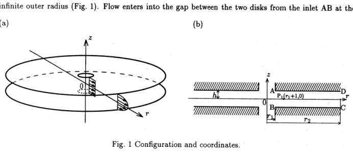
Consider aradiallyoutgoing_{flow between two parallel circular disks with the spacing} $2h^{*}$ and the

infinite outer radius (Fig. 1). Flow enters into the

gap

between the two disks from the inlet AB at the

(a) _(b)

Fig. 1Configuration and coordinates.

inner radius $r_{1}^{*}$ with auniform velocity profile. We define two non-dimensional

parameters, i.e., the

Reynolds number and the non-dimensional inlet radius, as

$Re \equiv\frac{Q^{*}}{4\pi\nu h^{*}}$,

$r_{1}\overline{=}r_{1}^{*}/h^{*}$, (1)

where $Q^{*}$ is the volumetricflow rate through the gap between two disks and

$\nu$ isthe kinematic viscosity

ofthe fluid.

2.1 Fundamental equation

Weintroduce the stream function $\psi(r, z, t)$ for the axisymmetric flow in the cylindricalcoordinates.

The governing equations for the vorticity component $\omega(r, z, t)$ in the circumferential direction and the

stream function $\psi(r, z, t)$ are written in anon-dimensional form as

$\frac{\partial\omega}{\partial t}-\frac{1}{r}\frac{\partial(\psi,\omega)}{\partial(r,z)}-\frac{1}{r^{2}}\frac{\partial\psi}{\partial z}\omega$ $= \frac{1}{Re}\Delta\omega$, (2)

$\omega=\frac{1}{r}D^{2}\psi$, (3)

where

$\frac{\partial(f,g)}{\partial(r,z)}\equiv\frac{\partial f}{\partial r}\frac{\partial g}{\partial z}-\frac{\partial f}{\partial z}\frac{\partial g}{\partial r}$ , $\Delta\equiv\frac{\partial^{2}}{\partial r^{2}}+\frac{1}{r}\frac{\partial}{\partial r}+\frac{\partial^{2}}{\partial z^{2}}-\frac{1}{r^{2}}$ , $D^{2} \equiv\frac{\partial^{2}}{\partial r^{2}}-\frac{1}{r}\frac{\partial}{\partial r}+\frac{\partial^{2}}{\partial z^{2}}$,

and all the physical variables are made non-dimensionalby using the representative length $h^{*}$ and the

representative velocity $Q^{*}/4\pi h^{*2}$

.

The flow is assumed to enter the inlet (AB in Fig. 1) with auniform velocity profile so that the

boundary condition is written as

$\psi=z$, $\omega=0$, $(r=r_{1})$. (4)

The boundary condition at the twodisks isthe nonslip boundary condition that is expressed by

$\psi=\pm 1$, $\omega=\frac{1}{r}\frac{\partial^{2}\psi}{\partial z^{2}}$

, $(z=\pm 1)$, ₍₅₎

where the complex signs are taken in the same order. The flow field is assumed to extend to infinitely

large radius, therefore the flow field has the asymptotic velocity at sufficiently large distance from the

center, whichisderived inthe next subsection. Then the boundary condition at the end of computational

domain (CD in Fig. 1) is expressed as

$\psi=\frac{1}{2}(3z-z^{3})+\frac{3}{8Re}(\frac{1}{7}z-\frac{11}{35}z^{3}+\frac{1}{5}z^{5}-\frac{1}{35}z^{7})\frac{1}{r^{2}}$,

$\omega$ $= \frac{3}{Re}(\frac{1}{7}z-\frac{11}{35}z^{3}+\frac{1}{5}z^{5}-\frac{1}{35}z^{7})\frac{1}{r^{5}}-3\frac{z}{r}+\frac{3}{4Re}(-\frac{33}{35}z+2z^{3}-\frac{3}{5}z^{5})\frac{1}{r^{3}}$,

$(r=r_{2})$. (6)

2.2 Asymptotic solutionfor far field

It is expected that the outgoing flow between two disks approaches to the fully developed plane

Poiseuille flow far downstream. We make an asymptotic analysis to derive the profile of the flow field at

far distance. Anew variabledefined by

$\xi=\frac{1}{r}$, (7)

is introduced, then the flow region is transformed from $r$ $=[r_{1}, \infty)$ to $\xi=[0,1/r_{1}]$

.

Steady flow field is

assumed at very far distance, therefore Eqs. (2) and (3) are rewritten as

$\xi^{3}\frac{\partial\psi}{\partial\xi}\frac{\partial}{\partial z}\Lambda\psi-\xi^{3}\frac{\partial}{\partial\xi}\Lambda\psi-\xi^{2}\frac{\partial\psi}{\partial z}\Lambda\psi=\frac{1}{Re}\Lambda^{2}\psi$, (8)

at fardownstream, where

$\Lambda=\xi^{4}\frac{\partial^{2}}{\partial\xi^{2}}+3\xi^{2}\frac{\partial}{\partial\xi}+\frac{\partial^{2}}{\partial z^{2}}$

.

We explore the solution $\psi(\xi, z)$ of Eq. (8) in aseries of expansionin$\xi(=1/r)$ expressed as

$\psi(\xi, z)=\psi_{0}+\xi\psi_{1}+\xi^{2}\psi_{2}+O(\xi^{3})$, (9)

where only the terms up to $O(\xi^{2})$ are retained. The boundary conditions for the expansion coefficients

$\psi_{n}$ are written as

$\psi_{0}=\pm 1$, $\frac{\partial\psi_{0}}{\partial z}=0$, $(z=\pm 1)$,

$\psi_{n}=0$, $\frac{\partial\psi_{n}}{\partial z}=0$, $(z=\pm 1)$, (10)

where the complex signs should be taken in the same order and $n$ should taken to be 1or 2. By

substituting the expansion (9) into Eq. (8) andequating the terms with the

same

power of4, we obtain

the equationsfor $\psi_{n}$, $(n =0,1,2)$

.

After solving the resultant equation for$\psi_{n}$, we obtain the asymptotic

expression of$\psi$ at large distance asexpressed as

$\psi(r, z)=\frac{1}{2}(3z-z^{3})+\frac{3}{8Re}(\frac{1}{7}z-\frac{11}{35}z^{3}+\frac{1}{5}z^{5}-\frac{1}{35}z^{7})\frac{1}{r^{2}}$

.

(11)

where the solutions are expressed in $r$by substituting $r$$=1/\xi$

.

The asymptotic solution (11) is adopted

astheboundarycondition forournumerical simulations and thenumerical calculationsofthe steady and

symmetric solutions

2.3 Steady and symmetric solution

Steady and symmetricsolution along the centerline between two disksexists regardless of the

mag-nitude ofthe Reynolds number, which is unstable at the Reynolds numbers above acritical value. The

steady and symmetricsolution$(\overline{\psi},\overline{\omega})$satisfies the steady-state equations, whichareobtained bydropping

the terms with time derivative$\partial/\partial t$ in Eq. (2).

The steady and symmetric solutioncan be calculated in the upper or lower half domain ofABCD

in Fig. 1therefore the boundary conditionon the centerline between the two disks is expressed as

$\overline{\psi}=0$, $\overline{\omega}=0$, $(z=0)$

.

(12)

The boundary conditions for $(\overline{\psi},\overline{\omega})$ at the inlet

$r=r_{1}$, the outlet$r=r_{2}$ andthe top orthe bottom disks

are the same as that of Eqs. (2) and (3).

2.4 Disturbance equation

We consider adisturbance $(\psi’, \omega’)$ added to the steady and symmetric solution $(\overline{\psi},\overline{\omega})$ and express

the stream function and the vorticity $(\psi, \omega)$ as $\psi=\overline{\psi}+\psi’$ and $\omega$ $=\overline{\omega}+\omega’$ to investigate the stability

of the steady and symmetric solution. The linear disturbance equations are obtained by substituting

the expressions for $\psi=\overline{\psi}+\psi’$ and $\omega$ $=\overline{\omega}+\omega’$ into Eqs. (2) and (3), subtracting the steady-state

equations, and neglecting the higher order terms than the linear terms concerning the disturbance $\psi’$

and $\omega’$. Furthermore, the solution

$(\psi’, \omega’)$ can be shown to have the form of $\psi’=\hat{\psi}\exp(\lambda t)$, and

$\omega’=\hat{\omega}\exp(\lambda t)$, then substitution of these expression into $(\psi’, \omega’)$ leads the equations for $(\hat{\psi},\hat{\omega})$ as

$\lambda\hat{\omega}-\frac{1}{r}\{\frac{\partial\overline{\psi}}{\partial r}\frac{\partial\hat{\omega}}{\partial z}+\frac{\partial\hat{\psi}}{\partial r}\frac{\partial\overline{\omega}}{\partial z}-\frac{\partial\overline{\psi}}{\partial z}\frac{\partial\hat{\omega}}{\partial r}-\frac{\partial\hat{\psi}}{\partial z}\frac{\partial\overline{\omega}}{\partial r}\}-\frac{1}{r^{2}}\{\frac{\partial\overline{\psi}}{\partial z}\hat{\omega}+\frac{\partial\hat{\psi}}{\partial z}\overline{\omega}\}=\frac{1}{Re}\Delta\hat{\omega}$, (13)

$\hat{\omega}=\frac{1}{r}D^{2}\hat{\psi}$. (14)

The boundary conditionsfor $(\hat{\psi},\hat{\omega})$ are written as

$\hat{\psi}=0$, $\hat{\omega}=0$, _{$(r=r_{1}, r_{2})$},

$\hat{\psi}=0$, $\hat{\omega}=\frac{1}{r}\frac{\partial^{2}\hat{\psi}}{\partial z^{2}}$

, $(z=\pm 1)$

.

(15)

The disturbance equation can be soIved in the upper or lower halfdomainofABCD in Fig. 1therefore

the boundary conditionon the centerline between the two disks isexpressed as

$\hat{\psi}(r, z)=\hat{\psi}(r, -z)$, $\hat{\omega}(r, z)=\hat{\omega}(r, -z)$, $(z=0)$

.

(16)

3. Numerical method

3.1 Numerical simulation

In numerical simulations by the time marching method, anequally spaced mesh system with $\Delta r=$

$\Delta z=5\cross 10^{-2}$ is used. The vorticity transport equation is solved by the Runge-Kutta method with

the fourth-0rder accuracy in time together with the second-0rder accuracy ofcentral finite difference in

space. The time increment At ischosen as $\Delta t=1\cross 10^{-4}$. The Poisson equation is discretized by the

second-0rder central finite difference and solved by the SOR method, where the relaxation factor $\epsilon$ is

taken as $\epsilon=1.82$

3.2 Steady and _{symmetric solution and linear stability analysis}

Both the steady-state vorticity transport equation and the Poisson equation are solved by the SOR

iterative method to calculatesteady and symmetric_{solutions. Spatial derivatives areapproximated by the}

second-0rder finite differences. The relaxation factor$\epsilon$ forthe SORmethodisdetermined by considering

the aspect ratio and the Reynolds number in the range $0.1<\epsilon<1.0$

.

_{In order to calculate unstable}

steady and symmetric solutions above acriticalReynoldsnumber, the SORmethod isutilized under the

symmetry conditionalongthe centerline between two disks. This method is used also for the numerical

evaluation of the linear growth rate.

4. Numerical results

4.1 Flow patterns and bifurcation

(a) _(b)

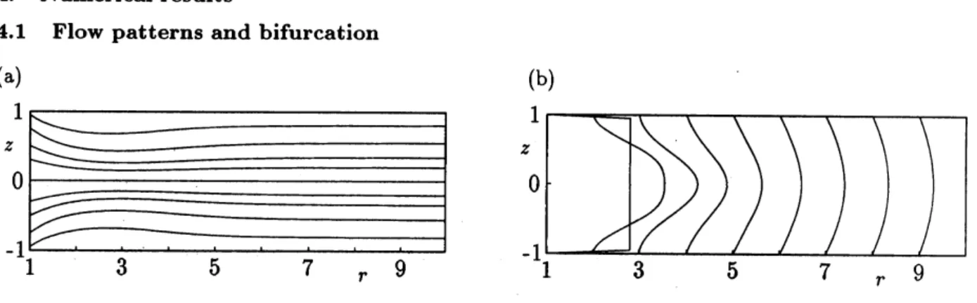
Fig. 2Flow pattern. $Re=40$,$r_{1}=1$

.

(a) Streamlines, (b) Velocity profiles.

For thecase ofthe non-dimensional inlet radius$r_{1}$ $=1$, we have done numericalsimulationsfor the

Reynolds numbers in the range of $10\leq Re\leq 200$

.

The outgoing flow is symmetric _{at small Reynolds}

numbers. Atypical example of such asteady and symmetric flow is shown in Fig. 2for $Re=40$.

Streamlines for the symmetric flow is depicted in Fig. 2(a) and the velocity profiles in the z-direction

isshown in Fig. 2(b). The streamlines gather together just downstream ofthe inlet as seen in Fig. 2

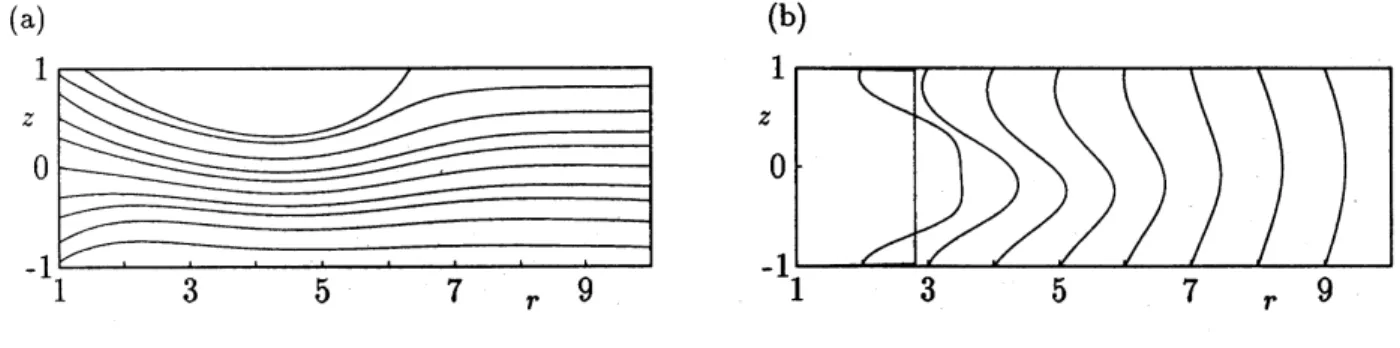
(a), where jet-like flow is observed in Fig. 2(b). Another flow pattern shown in Fig. 3 $(Re=50)$ is

also asteady and symmetricflow, but differs from that in Fig. 2in presence of separation vortices. The

separation vortices in Fig. 3(a) are formed lying in $r$ $=1.85-3.55$near both the upper andlower walls.

(a) (b)

Fig. 3Flow pattern. $Re=50$,$r_{1}=1$

.

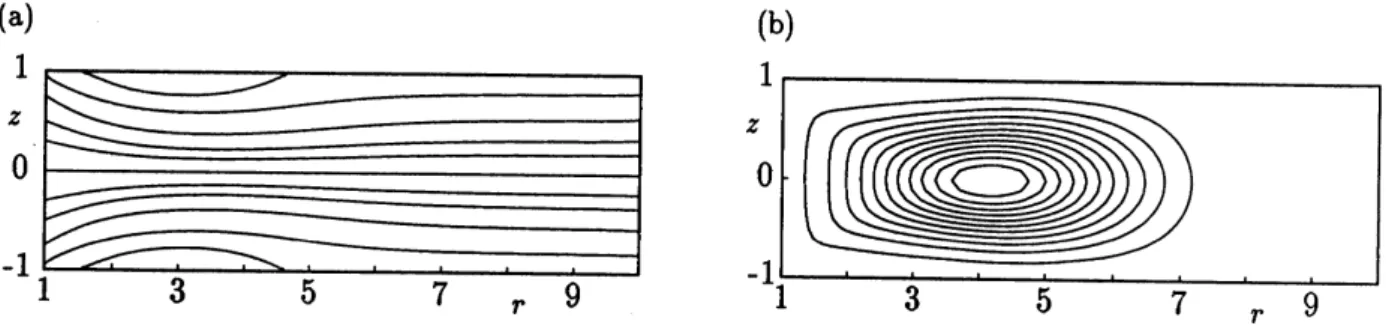
(a) Streamlines, (b) Velocity profiles.

The flowpatternobtainedinnumericalsimulations at$Re=70$_issteady, butasymmetricas depicted

in Fig. 4. The stream coming from the inlet is seen to bend on the lower wall. We can easily imagine

another asymmetric flow, which bendson the upper wall from thesymmetryconsideration of the system.

Such asteady and asymmetric flow has not been reported _{before. The separation-vortex region in Fig. 4}

(a) (b)

Fig. 4Flow pattern. $Re=70$,$r_{1}=1$

.

(a) Streamlines, (b) Velocity profiles.

(a) is larger than that in Fig. 3(a), and the separation vortexlies in $r=1.5-6.3$near the upper wall.

Fig. 5Bifurcation diagram, $r_{1}=1$.

We have confirmed by numerical calculations of the steady-state equationsthat the symmetric flow

also does exist at $Re=70$. The asymmetric flow is thought to appear due to the instability of the

symmetricflow. In order to investigatethebifurcation ofsteady-state solution,weobtainthe bifurcation

diagram by adopting arepresentation value $v_{1}$, the velocity in $z$-direction at arepresentation point $\mathrm{P}_{1}$

$[(r, z)=(2, \mathrm{O}),\mathrm{F}\mathrm{i}\mathrm{g}.1]$. The bifurcation diagram is depicted in Fig. 5. The bifurcation is determined as

apitchfork bifurcation from the relation $v_{1}^{2}\propto$ $(Re -Re_{\mathrm{c}})$, and the critical Reynolds number $Re_{\mathrm{c}}$ being

62.7.

4.2 Linear stability analysis

We investigatethe linearstability ofthe steady and symmetric solution whichis abasic solution of

theoutgoingflowfor thecaseof thenon-dimensionalinlet radius $r_{1}=1$. We have solved the steady-state

equations numerically to obtain the steady andsymmetricsolutions $(\overline{\psi},\overline{\omega})$ and also solved Eqs. (13) and

(14) to evaluate the lineargrowth rate Afor the steady andsymmetricsolutions. Typical examples ofa

steadyandsymmetricflowandalineardisturbance areshownin Fig. 6forthe Reynolds number$Re=64$.

Figure 6(a) shows the streamlines of the steady and symmetricsolution, and the disturbance obtained

by solving Eqs. (13) and (14) is depicted in Fig. 6(b). The disturbance hassignificant magnitude in a

(a) _(b)

Fig. 6Flow pattern. $Re=64$,$r_{1}=1$

.

Streamlines, (a) Unstable_{symmetricflow, (b) Disturbance,}

limited region

near

the inlet, which makes thesymmetric_{flow to bend on one wall in that region.}

Fig. 7Linear growth rate $\lambda$,

$r_{1}$ $=1$

.

Thelinear growth rate Ais evaluated forvariousReynoldsnumbers, whichisshown in Fig. 7for the

non-dimensionalinlet radius$r_{1}=1$

.

The critical Reynoldsnumber$Re_{\mathrm{c}}$ is determined as $Re_{\mathrm{c}}=62.8$from

Fig. 7for the non-dimensionalinlet radius $r_{1}=1$

.

The relative

error

between the values of $Re_{\mathrm{c}}=62.7$

obtained from the bifurcation diagramand $Re_{\mathrm{c}}=62.8$from the linear stability analysis is about 0.16%,

which shows the consistency between the two values.

We have evaluated the critical Reynolds number $Re_{\mathrm{c}}$ for others values of the non-dimensional inlet

radus$r_{1}$ and depicted themagainst$r_{1}$ inFig. 8in therangeof$0.5\leq r_{1}$ $\leq 3$

.

The flowissymmetric atthe

Reynolds number under the solid line in Fig. 8, but becomes asymmetricat the Reynoldsnumber above

the line. The steady and asymmetricflow may make atransition into an oscillatoryflow above another

Reynolds number, say $Re_{\mathrm{c}}’$

.

However, it may be possible that the steady and

symmetric flow makes a

transition into anoscillatory flow without experiencing anasymmetric_{flow for the non-dimensionalinlet}

radii $r_{1}$ much larger than 3. The critical Reynolds number $Re_{\mathrm{c}}’$ mayapproach to 5771, where the plane

Poiseuille flow becomes unstable

Fig. 8Critical Reynolds number and $r_{1}$ : the non-dimensional inlet radus.

5. Conclusions

We made an asymptotic analysis for the flow profile at far distance and confirmed the flow field

approaches to the fully developed plane Poiseuille flow there. We have done numerical simulations,

numerical calculations of the steadysymmetric solutions and their linear stabilityanalysisfor theoutgoing

flow with finite difference approximations. As results, we found that the flow is symmetric at small

Reynolds numbers, but becomes asymmetric above acritical Reynoldsnumber. The transition into the

asymmetric flow is determineddue to apitchfork bifurcation judging fromthe relation $v_{1}^{2}\propto(Re-62.7)$

for the non-dimensional inlet radius $r_{1}=1$

.

The critical Reynolds number obtained from the linear

stability analysis is62.8 which is in good agreement with the critical value62.7 evaluated by numerical

simulationdata. Thelarger the value of the non-dimensional inlet radii $r_{1}$ is, the largerthe valueof the

critical Reynolds numbers $Re_{\mathrm{c}}$ for atransition into asymmetricflow becomes.

References

1) S. Ishizawa, Bulletin of JSME, 8, 353-367 (1965).

2) S. Ishizawa, Bulletin ofJSME, 9, 86-103 (1966).

3) J. D. Raal, J. Fluid Mech., 85, 401-416 (1978).

4) S. Mochizuki and W. J. Yang, J. Fluid Mech., 154, 377-397 (1985)